TCP

The Transport Layer #

The transport layer (L4) is built directly on top of the networking layer. Many different protocols exist on the transport layer, most notably TCP and UDP. (For the security perspective — TCP injection, RST attacks, and how TLS sits on top of TCP — see Networking.)

The goal of the transport layer is to bridge the gap between the abstractions application designers want, and the abstractions that networks can easily support. By providing a common implementation, the transport layer makes development easier.

The main tasks of the transport layer include:

• Demultiplexing (taking a single stream of data and identifying which app it belongs to)
  • Port numbers carried in L4 protocol header
• Providing reliability
• Translating from packets to app-level abstractions
• Avoid overloading the receiver (flow control)
• Avoid overloading the network

TCP Segments #

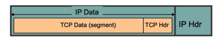
Individual bytes in the bytestream are divided into segments, which are sent inside of a packet. (A TCP packet is just an IP packet whose data contains a TCP header and segment data.)

The maximum segment size (MSS) is equal to the MTU - (size of IP header) - (size of TCP header).

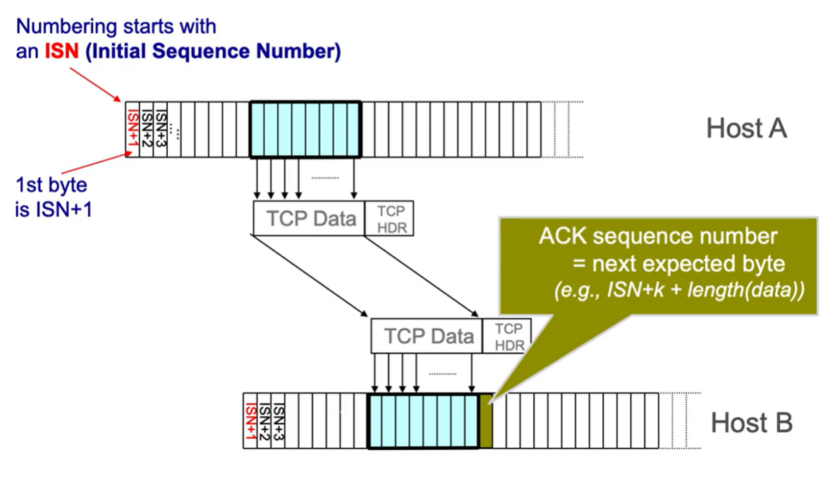
TCP Sequence Numbers #

Important: TCP operates on bytes, not packets. Sequence numbers, ACKs, window sizes, etc. are all expressed in terms of bytes.

TCP Properties #

TCP is connection oriented #

TCP requires keeping state both on the sender and the receiver.

• Sender keeps track of packets sent but not ACKed, and any timers needed for resending.
• Receiver keeps track of out-of-order packets.

Each bytestream is called a connection or session, each with their own connection state stored at end hosts.

TCP connections are full-duplex #

If Host A and Host B are connected via TCP, hosts A and B can both be senders and receivers simultaneously. This means that Host A and Host B can be sending and receiving from each other using the same connections.

Reliability handling #

• Sequence numbers are byte offsets
• TCP uses cumulative ACKs (next expected byte: the sequence number of the next packet is the same as the last ack)
• Sliding window that allows up to $W$ contiguous bytes to be in flight at the same time
• Retransmissions are triggered both by timeouts and duplicate acks
• Single timer is used for the 1st byte of the window
• Timeouts computed from RTT measurements

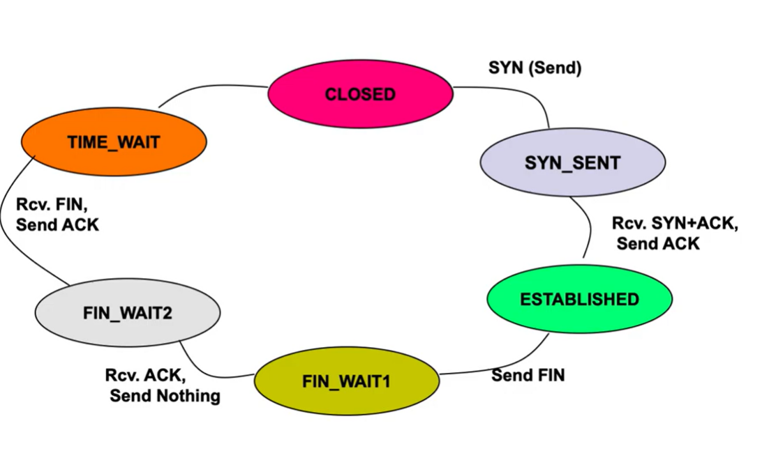
TCP States #

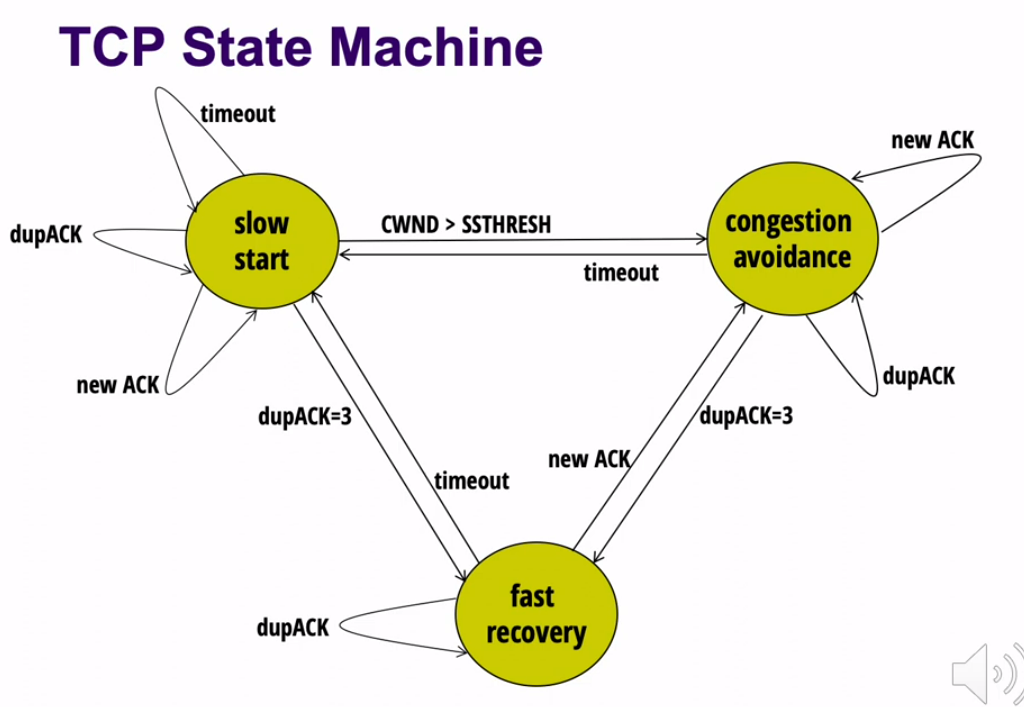
Congestion Control Implementation #

For an intro to congestion control, see congestion control.

TCP uses a loss-based, host-based, dynamic adjustment congestion control scheme.

Terms #

• Loss-based: window determined by packet loss
• Host-based: routers do not participate; window size is implicitly determined by hosts only
• AIMD: Additive Increase Multiplicative Decrease
• RWND: Advertised window/Receiver window: maintained by receiver and directly communicated to sender for flow control (max bandwidth the receiver can handle before buffer overflow)
• CWND: Congestion Window: computed by sender using concurrency control algorithm (how many bytes can be sent without overloading links)
• Sender-side window: min of RNWD and CWND. Typically, assume that RWND » CWND.
• MSS: Maximum Segment Size: max number of bytes of data that one TCP packet can carry in payload
• Sender Transmission Rate: CWND/RTT (bits per second)
  • Changing CWND <==> changing transmission rate
• SSTHRESH: slow start threshold (last safe rate). equal to CWND/2 on first loss

Window Mechanics #

Recall that the sender maintains a sliding window of $W$ contiguous bytes, where $W$ is the window size (typically CWND). On receiving an ACK for new data $j$ where $j>i$, then the window slides to start at $j$.

The sender maintains a single timer for the smallest value $i$ in the window. On a timeout, the sender retransmits the packet that starts at byte $i$.

Since the receiver sends cumulative ACKs, full information isn’t provided so the sender will count the number of duplicate acks received (dupACK). When dupACK == 3, the sender will retransmit (fast retransmit).

Changing CWND #

Main idea: Change CWND based on ACK arrivals (ack clocking)

• The spacing between acks is representative of the bandwidth. Longer spacing = lower bandwidth
• Optimal solution = full utilization of minimum link bandwidth

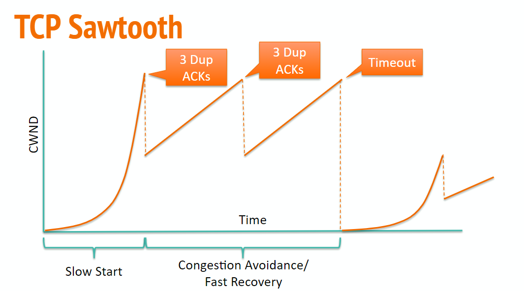
Slow Start #

1. Initialize CWND equal to MSS. (initial sending rate is one MSS per RTT)
2. Double CWND every RTT until first loss occurs. (On every ACK, add 1x MSS to CWND)
3. When first loss occurs, set SSTHRESH=CWND/2

AIMD/Congestion Avoidance #

• No loss -> increase CWND by 1 MSS every RTT
  • Implementation: successful ACK received ->$CWND = CWND + MSS \times MSS/CWND$
• 3 dupACK -> divide CWND in half
  • Implementation: save dupACKcount in memory, and increment if duplicate detected
• Timeout -> set CWND to MSS, and restart Slow Start
  • switch back to AIMD when SSTHRESH is hit

Fast Recovery #

Fast Recovery is an optimization to congestion avoidance. The main idea is to keep packets in flight by allowing senders to keep sending even when a dupACK is received.

If dupACKcount is 3:

• set SSTHRESH to $\lfloor CWND/2 \rfloor$
• set CWND to SSTHRESH + 3xMSS

While in fast recovery:

• CWND = CWND + MSS for every additional dupACK
• Set CWND = SSTHRESH upon receiving first new ACK

State Machine #

TCP Sawtooth

TCP Throughput #

Given RTT and the loss rate $p$, we can derive the throughput of TCP.

Assume:

• loss occurs whenever CWND reaches $W_{max}$
• loss is detected by duplicate ACKS (no timeouts)
• ignore slow start throughput

Since we go between half of $W_{max}$ and full, the average window size per RTT is equal to $\frac{3}{4}W_{max}$. Therefore, the average throughput is $\frac{3}{4}W_{max} \times \frac{MSS}{RTT}$. 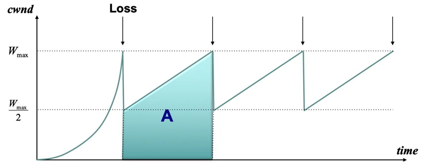On average, our loss rate is $p=1/A$ (where A Is the area under the curve in one of the periods). Using this, we can see that the area $A$ is equal to $\frac{3}{8}W_{max}^2$.

Solving for $W_{max}$ and plugging it into the average throughput equation yields this formula for average throughput:

Implications of throughput equation #

• Flows get throughput inversely proportional to RTT. So lower RTT = higher throughput, which can be unfair for further connections.
• Scaling a single flow to high throughput is very slow with additive increase, and ramping up to very fast bandwidth (hundreds of gbps) could take hours.
  • solution: HighSpeed TCP (RFC 3649): past a certain threshold speed, increase CWND faster.
• TCP throughput is choppy due to repeated swings: some apps (streaming) may prefer sending at a steady rate
  • solution: equation-based congestion control (measure RTT and drop percentage $p$ and directly apply equation)
• TCP confuses corruption with congestion: throughput is proportional to 1/sqrt(p) even for non-congestion losses
• Due to 50% of flows being <1500B, many flows never leave slow starts, and there are too few packets to trigger dupACKs
  • solution: use higher initial CWND
• since TCP fills up queues before detecting loss, delays can be large for everyone in a bottleneck link
  • solution: Google BBR algorithm (sender learns minimum RTT, and decreases rate when observed RTT exceeds minimum RTT)
• congestion control is intertwined with reliability: CWND is adjusted based on acks and timeouts. we can’t easily get congestion control without reliability.

Fairness #

General approach:

• A router classifies incoming packets into flows.
• Each flow has its own queue in the router.
• The router picks a queue in a fair order and transmits packets from the front of that queue.

Max-Min Fairness #

Main idea: if a flow doesn’t get its full demand, then no other flow will get more than that amount.

If the total available bandwidth is $C$ and each flow $i$ has a bandwidth demand $r_i$, then the fair allocation of bandwidth $a_i$ to each flow is calculated as

where $f$ is the flow’s fair share, calculated by the following:

• Get the average $C/N$ (where $N$ is the number of flows).
• Subtract all of the $r_i$ from $C$ where $r_i < N$. For each flow that this is done for, subtract one from $N$.
• For all of the remaining flows, set $f = C/N$.

Fair Queueing (RCP) #

FQ addresses the issue where packets may not all be the same size.

• For each packet, compute the time where the last bit would have left the router if flows are served bit by bit (deadlines)
• Serve packets in increasing order of their deadlines.

Advantages of FQ:

• Isolation of flows (cheating flows don’t benefit)
• bandwidth share does not depend on RTT
• flows can pick any rate adjustment scheme

Disadvantages:

• more complex than FIFO
• only helps, but does not solve, congestion control
• too complex to implement at high speeds
• unfair for applications with different numbers of flows

Explicit Congestion Notification (ECN) #

• Single bit in packet header set by congested routers in ACK
• Host treats acks with set ECN bit as a dropped packet
• Doesn’t confuse corruption with congestion
• Early indicator of congestion can be used to avoid delays
• lightweight to implement