Fast Fourier Transform (FFT)

Polynomial Multiplication #

The Problem #

Let’s say we have two input polynomials $A(x) = \sum_{i=0}^d a_ix^i$ and $B(x) = \sum_{i=0}^d b_ix^i$.

We would like to find an output $C(x) = A(x) \cdot B(x)$. $C(x)$ has a degree $2d$.

By definition of polynomial multiplication,

Let’s gather all of the coefficients with the same power together to make this expression more useful:

The naive algorithm #

Let’s just follow the definition and evaluate each term one by one, from $i=0$ to $i=2d$.

• The outer loop has $2d$ iterations.
• The inner loop has runtimes that sum from $1$ to $2d$ as a result of the outer loop.

This means that the runtime for the naive algorithm is $O(d^2)$.

Improving the algorithm #

Observation: If we want to evaluate polynomials (find $C(u)$ at a point $u$), we can do so with a single multiplication of $A(u)$ and $B(u)$. We can use this to come up with something interesting:

1. Evaluate $A(u)$ and $B(u)$ on many points.
2. Pointwise multiply $A$ and $B$ to get the value of $C(u)$.
3. If we have enough, then we can use polynomial interpolation to get a unique expression for $C$.

Polynomial Interpolation #

So… how do we actually do that third step?

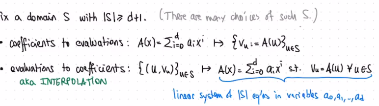
Recall that any degree $d$ polynomial can be reconstructed by $d+1$ points from that polynomial. This creates two representations of polynomials, the evaluation representation and the coefficient representation:

The Algorithm #

Let’s multiply $A(x)$ with $B(x)$ now:

1. Choose a domain of points $S$ with $S \ge 2d+1$ (such that we can guarantee unique reconstruction of $C(x)$).
2. Evaluate $A(u)$ for all $u \in S$.
3. Evaluate $B(u)$ for all $u \in S$.
4. Compute $C(u) = A(u)B(u)$ for all $u \in S$.
5. Interpolate $\{u, c(u)\}_{u \in S}$

The runtime of this algorithm will be $2T_{eval}(d) + O(d) + T_{interp}(2d)$ where $T_{eval}$ is the time it takes to evaluate a degree $d$ polynomial (steps 2 and 3) and $T_{interp}$ is the time it takes to interpolate a polynomial of degree $2d$.

We still haven’t seen how to actually evaluate and interpolate the polynomials in the first place though- but we will now!

The Fast Fourier Transform #

The Main Idea #

Make a clever choice of the set of points $S$ such that we can use divide and conquer to evaluate a polynomial in smaller and smaller domain sizes.

A natural way to split up a polynomial into two smaller polynomials is to get only the odd power terms, or only the even power terms.

So, we can rewrite a polynomial $A(x)$ as $A_e(x^2) + x \cdot A_o(x^2)$ where $A_e$ is all even terms (including the constant term) and $A_o$ is all odd terms with one $x$ factored out (such that the terms end up being even too).

In order to make this work, we need to choose an $S$ such that $S^2$ has a size $S/2$. But how can we do this??

Roots of Unity #

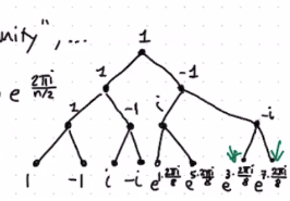
We can notice that if we choose $\{1, -1\}$, then $S$ has two elements but $S^2$ only has one since $(-1)^2 = 1$. This is a start, but we need to consider arbitrarily large $S$. We can’t just add more positive and negative numbers since only $1$ and $-1$ are guaranteed to have this property, so we need to start considering complex numbers.

A key to this is the roots of unity: the solutions to the equation $x^n = 1$. In order to find these, we walk around the unit circle on the complex plane:

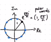
Recall that $e^{\pi i} = -1$ and $e^{2\pi i} = 1$. This means that a number $\alpha$ has the same square as $\alpha \cdot e^{\pi i}$, analogously to the $1, -1$ example above. If we choose enough $\alpha$, then we can get $2d+1$ points pretty easily!

The FFT algorithm #

For this section, let $\omega = e^{2\pi i / n}$ for convenience.

What the algorithm does: Given a polynomial $A(x)$, output $A(\omega^0), \cdots A(\omega^{n-1})$ where $n$ is the smallest power of 2 greater than the number of terms in $A$.

Step 1: Split $A(x)$ into even and odd polynomials, $A_e(x)$ and $A_o(x)$.

Step 2: Recursively evaluate the FFT of $A_e(x)$.

Step 3: Recursively evaluate the FFT of $A_o(x)$.

Step 4: Sum up the terms of $A_e(x)$ and $A_o(x)$. This reduces the problem size because $A_e(x^2) + x \cdot A_o(x^2) = A(x)$. Since we chose a set $S$ such that $|S^2| = |S|/2$, both of these evaluate to the same thing.

The runtime of FFT is $T(n) = 2T(n/2) + O(n)$.

By the Master Theorem with $a=2, b=2, d=1$, this is a balanced tree so $O(n^d\log_2(n)) = O(n\log(n))$.

https://www.youtube.com/watch?v=h7apO7q16V0