Graphs

Graph Representations #

A graph is a pair $(V,E)$ where $V$ is the vertex set and $E \subseteq V \times V$ is the edge set. (For an introductory data-structures treatment, see graphs; for the discrete-math/combinatorial properties used in proofs, see graphs.)

There are 2 main ways to represent graphs for an algorithm:

Adjacency Matrix #

$M_G = \begin{pmatrix} m_{ij} \end{pmatrix} \in \{0,1\}^{m \times n}$

If $m_{ij} = 1$, then that means the vertices $i$ and $j$ are connected with an edge.

Adjacency List #

$L_G = 1 \to 3, 5, 7, 11 \cdots$ $2 \to 5, 8, 9 \cdots$

A list of lists: each list is the connections from one vertex to others.

Tradeoffs #

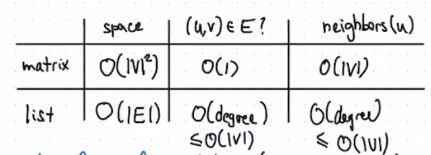
Space: In a matrix, we have $|V|^2$ number of entries (since the matrix is $V \times V$). On the other hand, a list has $O(|E|)$ number of entries. Therefore the list is better for sparce graphs (lots of vertices, few edges).

isConnected query: If we want to determine if two vertices are connected:

A matrix will allow $O(1)$ time queries since we can simply read off the $m_{ij}$ element.
A list requires $O(|V|)$, or more specifically, the order of the degree of the vertices since we need to iterate over all of the connections on one of the vertices to see if the other is contained.

getNeighbors query: If we want to find all of the neighbors (connections) of a vertex:

A matrix requires $O(|V|)$ since we need to iterate over a row in the matrix.
A list is again $O(degree)$ for the same reason as isConnected.

Graph Traversals #

The Explore Procedure #

def explore(G, v):
	visited[v] = true
	for each (v, u) in E:
		if not visited[u]:
			explore(G, u)

Claim: This procedure visits every vertex reachable from $v$.

Proof:
Proof by contradiction:
Suppose that there exists a vertex $a \in V$ that is reachable from $v$ but not visited by explore.
Then, there exists a path $v, \cdots w, z, \cdots a$ where $w$ is the last visited node, and $z$ is the first unvisited node that is adjacent to $z$.
But if $w$ is visited, we must have run explore(G, w) which is guaranteed to visit $z$. Therefore, it is impossible for $z$ to have not been visited, and so $z$ does not exist and this is a contradiction.

Depth First Search (DFS) #

visited = [False for v in V]
for each v in V:
	if not visited[v]:
		explore(G, v)

Unlike explore by itself, DFS is guaranteed to visit every vertex in the graph, even if they are not connected.

Runtime Analysis:

Every directed (outgoing) edge is considered exactly once by explore. So, every undirected edge is considered twice (once by explore(G, i) and once by explore(G, j)).
DFS loops through every vertex to run explore on them.

Therefore, the runtime of DFS is O(|V| + |E|).

Time Tracking #

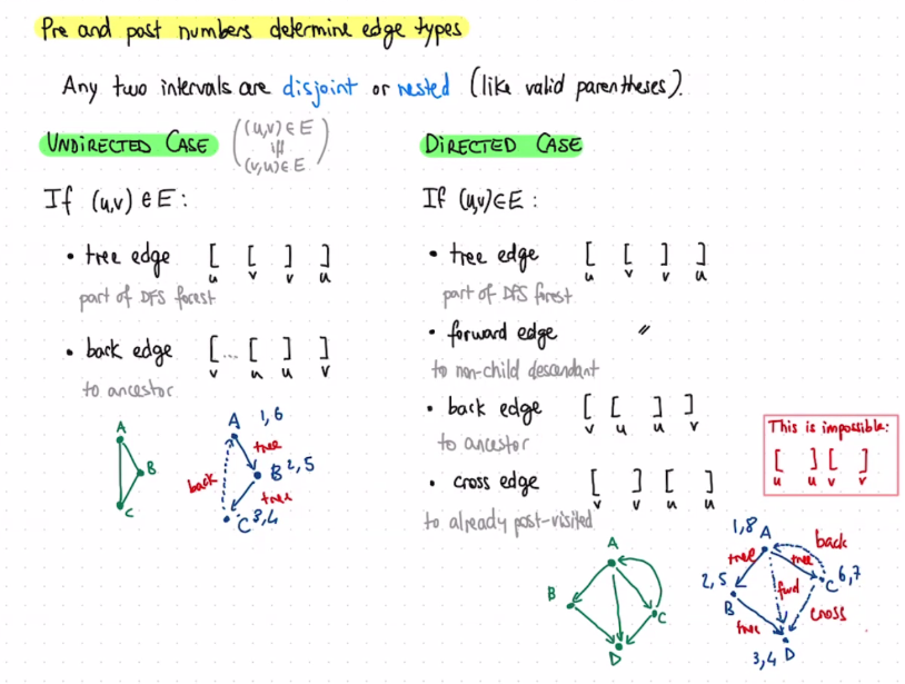
Suppose we want to figure out how long it takes to explore each vertex. Then, we can create a pre and post time stack. pre is incremented in explore before the for loop, and post is incremented after the for loop.

Directed Acyclic Graphs #

A graph is acyclic if it doesn’t have any cycles.

Claim: G is acyclic if and only if there are no back edges.

Proof:
Without loss of generality, suppose we visited $v_1$ first, and that G has a cycle $v_1, \cdots v_t$. Then, when $v_t$ is explored, it will cause a back edge from $v_t$ to $v_1$ because $v_1$ has already been visited.

The isDAG Algorithm

Run DFS(G) to collect pre and post numbers (see ’time tracking’ section).
For each edge (u, v), if (u, v) is a back edge then return False.
If there are no back edges, return True.

Note that we didn’t actually find the cycle, we only determined if there exists a cycle or not.

The runtime of this algorithm is the same as DFS: O(|V|+|E|).

Topological Sort #

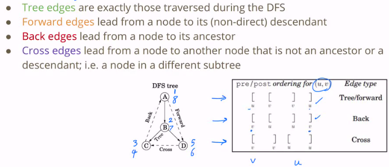
A topological sort of a direct acyclic graph is a total order on vertices such that each edge goes from an earlier vertex to a later one.

In other words, if we were to redraw the graph after topological sort in the order they were visited, all edges should point from left to right.

If a graph is directed and acyclic, then for all edges $(u, v)$ in depth first search, post[u] > post[v].

Proof:
Simple proof by contradiction: If post[v] > post[u] then by definition this is a back edge. Therefore, the graph has a cycle and it is not a DAG.

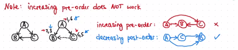
This fact leads to an algorithm for Topological Sort:

Run DFS(G) to collect pre- and post- numbers.
Ouput vertices in decreasing post order.

This runs in $O(|V|+|E|)$ time since the post orders don’t need to be sorted in step 2: they are already returned from DFS in order due to the fact above.

Connectivity #

We can use a modified DFS to determine all of the connected components (parts of the graph that are all connected).

Code:

visited = [False for v in V]
ccnum[v] = [None for v in V] # NEW: connected component number of each vertex

cc = 0 # NEW: current connected component
for each v in V:
	if not visited[v]:
		cc += 1 # NEW: Increment connected component if this vertex is not connected
		explore(G, v)

def explore(G, v):
	visited[v] = true
	ccnum[v] = cc # NEW: save component number
	for each (v, u) in E:
		if not visited[u]:
			explore(G, u)

Since we didn’t add any more iteration, the runtime is the same as DFS, $O(|V|+|E|)$.

A directed graph has two vertices $(u,v)$ that are strongly connected if there are two distinct paths, one from $u,v$ and another from $v,u$.

A strongly connected component is one where all of its vertices are strongly connected to each other. (These SCCs are guaranteed to have cycles.)

Every graph is a directed acyclic graph of strongly connected components.

Finding Strongly Connected Components #

Some ideas to get us started:

explore(G, v) visits all vertices reachable from a vertex $v$.
We can split vertices reachable from $v$ into two categories, source (actual SCC) and sink (where going to these vertices makes you get stuck, not SCC). If we can figure out what vertices are in the sink, we can remove them to get the SCC.

So, how do we find the sink?

Find $G^R$, the graph of $G$ with all its edges reversed. (This can be done in linear time)
Run $DFS(R)$ to get post numbers.
For each $v \in V$ in reverse post order:
1. If $v$ hasn’t been visited before:
  1. explore(G, v)
  2. Increment SCC number.

If we run explore starting inside a sink, then it will not be able to leave until the algorithm increments the $v$ in the for loop.

Graph Paths #

DFS is great for figuring out if a vertex is reachable, but tells us nothing about how long it takes to get there.

Let’s now explore some ways to get shortest paths in a graph. In other words, given a vertex $v$, find the distance (and path) from $v$ to all other vertices in the graph.

If we organize all vertices in sets corresponding to distances away from $v$ (i.e. $V_0 = \{v\},$ $V_1 =$neighbors of $v$, etc. then we can create a recursive algorithm to determine $V_{n+1}$ from $V_n$.

Notice that $V_{n+1}$ consists of all neighbors of vertices in $V_n$ other than the ones that have already been added to the set $V_{n-1}$.

Breadth First Search #

Code:

def BFS(G, s):
	dist[s] = 0 # starting
	for all other vertices v in G:
		dist[v] = infinity
	Q = priorityQueue
	add s to Q

	while Q is not empty:
		u = pop(Q)
		for every edge pair (u,v) in edges(G):
			if dist[v] = infinity: # we haven't seen v yet
				push(Q, v) # add to priority queue
				dist[v] = dist[u] + 1

Notice that in BFS, we use a Queue (FIFO), whereas in DFS we use a stack (LIFO).

Runtime Analysis:

Initializing the dist array is $O(|V|)$ since every vertex needs to be initialized.
Every vertex is pushed and popped from the queue exactly once, which takes $O(|V|)$ time.
Each edge is examined once, which takes $O(|E|)$ time.

Therefore, BFS takes $O(|V|+|E|)$ time like depth first search.

Dijkstra’s Algorithm #

💡 61b version: Dijkstra’s Algorithm

Up to this point, we’ve dealt with graphs where all edges have the same length. What happens if each edge has a different length? How will we solve the shortest paths problem now?

Main Idea: Continually add to a subgraph $K$. Everything inside $K$ is the shortest paths, and everything outside is not.

def dijkstra(G, s): # get shortest path to s from o
	dist[s] = 0
	for all vertices v that is not s:
		dist[v] = infinity
	U = vertices(G) # U = V \ K
	while U is not empty:
		pick u in U with smallest dist[u]
		U.remove(u)
		for all (u, v) in edges(G):
			dist[v] = min(dist[v], dist[u] + length(u, v))

Explanation:

Proof of Correctness:

Let $d(s,v)$ be the length of a shortest path from $s$ to $v$.

We must prove that $\forall v \in K,$ dist[v] = d(s,v).

We can prove this by induction:

Base case: If $K$ has a single vertex, then there is only one edge connecting $s$ and $v$ so the shortest path is trivial.
Induction step: Let $v$ be the vertex with the smallest dist[v]. As our inductive hypothesis, let’s say that dist[v] == d(s,v). Now, let’s consider a shortest path from $s$ to $v$. Suppose this shortest path contains a vertex $a$, but another vertex $b$ is not included in this path. As a fact, every sub-path (prefix) of a shortest path is also a shortest path! There are now two cases to consider:
- If $b = v$, then dist[v] = dist[b] = dist[a] + l(a,b) = d(s, a) + l(a, b)where l(a,b) is the edge connecting $a$ to $b$. Since $a$ and $b$ are adjacent by construction, $d(s,a)$ is a prefix of $d(s, b)$ and therefore dist[b] = dist[v] = d(s, b). This shows that $K$ contains the shortest path to $v$.
- If $b \ne v$, then this would be a contradiction because it would suggest that dist[a] is not the shortest path from $s$ to $a$. This conflicts with our inductive hypothesis so this case will never occur.

Runtime

Assuming we use a priority queue implementation:

Initializing the queue requires $|V|$ inserts (one for each vertex). This takes $O(|V| \log |V|)$ with a binary heap implementation, or $O(|V|)$ with a Fibonacci implementation.
We will need to delete each vertex once from $U$, which in total takes $O(|V|)$ time.
We must change dist[v] once per edge, which takes $O(|E|)$ time.

Overall, this takes $O((V + E) \log(V))$ time.

Bellman Ford: Shortest Paths with Negative Edge Lengths #

One shortcoming of Dijkstra’s algorithm is that it can’t handle a mixture of positive and negative edge lengths. (This is because a path A -> 100 -> -99 -> B is shorter than a path A -> 2 -> B, but Dijkstra’s will not check the first path until the end, when the rest of the graph has already been explored.)

In order to mitigate this, we can come up with a better updating algorithm that handles this. So rather than outright setting dist[v] = min(dist[v], dist[u] + length(u, v)) like in Dijkstra’s, we should:

Update a “safe” distance such that dist[v] >= d(s, v).
Doing additional updates to dist[v] is also considered “safe”, because an update always reduces the distance.
Do enough updates such that every possible update is done, so the true smallest dist[v] is included.

Here’s the Bellman-Ford Algorithm:

def BellmanFord(G, s):
	for i in range(1, |V|):
		for all (u, v) in edges(G):
			update(u, v)

def update(u, v):
	w = length(u, v)
	if distance[u] + w < distance[v]:
      dist[v] = dist[u] + w
      predecessor[v] = u

Runtime:

Bellman Ford requires nested iteration: the outer loop runs $|V| - 1$ times, and the inner loop runs once per edge, so $|E|$ times. Each run calls update once, which takes $O(1)$ time. Multiplying all of these together:

****$O((|V| - 1) \cdot |E| \cdot 1) = O(|V| \cdot |E|)$

Detecting Negative Cycles #

One issue to figure out is that of negative cycles: If we get stuck in one of these, then the longer we go around it then the smaller the length, with no limit to how small it can get. Currently, our implementation of Bellman-Ford only works if it is assumed that no negative cycles exist.

Proposal: Instead of running Bellman-Ford $|V| - 1$ times, let’s run it $|V|$ times. If dist[v] changes for any vertex, then a negative cycle exists.

Proof: If there are no negative cycles, then all shortest paths have at most $|V| - 1$ vertices. Therefore, updating one more time is considered “safe”: it should be impossible for any distances to decrease, because there are no more vertices to visit.

ben's notes