Linear Programming

What is Linear Programming? #

Linear programming is expressing and solving linear optimization, typically in higher dimension problems.

An optimization problem has the following form:

$n$ real variables $x_1, \cdots, x_n \in \mathbb{R}$,
An objective function $f(x_1, \cdots, x_r) \in \mathbb{R}$
$m$ constraints $c_1, \cdots c_m$ such that $c_i(x_1, \cdots, x_n)$ returns either true or false.
A goal to get the maximum of $f(x_1, \cdots, x_n)$ such that all constraints are true.

A linear programming problem is a subset of optimization problems, such that:

$f$ must be a linear function (i.e. a linear combination of variables scaled by constants).
Each constraint is a linear constraint (either an equality or inequality).
- For example, $5x_1 + x_2 \ge 0$ is a linear constraint.
All inequalities must be non-strict ($\ge, \le$ and not $>, <$) because otherwise it is possible for there to not be an optimal solution. (for example if we are trying to find the max of $x$ such that $x < 3$, we must take a limit to find the solution)

An example problem #

Bob is a salesperson trying to sell chestnuts and pretzels.

Chestnuts provide $2 profit and we can sell at most 50 of them.
Pretzels provide $4 profit and we can sell at most 80 of them.
There is a total space of 100 items in the cart.
We would like to maximize profit.

We can map this problem to an LP instance:

Variables: Let $x_1$ represent the number of chestnuts, and $x_2$ represent the number of pretzels.
Objective function: $f(x_1,x_2) = 2x_1 + 4x_2$ representing the profit.
Constraints:
- $x_1 \ge 0, x_2 \ge 0$
- $x_1 + x_2 \le 100$
- $x_1 \le 50$
- $x_2 \le 80$

One method of solving this problem is to draw it to find that the max input is $(20, 80)$.

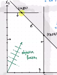
Geometric Observations #

The above problem was solvable using geometry. Here are some parallels between LP properties and their geometric equivalents:

An inequality → “half space” (cuts the total solution space into two)
Feasible solutions → Intersection of all half spaces created by inequalities
Objective function → direction
Optimal solution → Follow the objective function until it reaches the boundary of the feasible solution set.
- The set of feasible solutions can also be empty or unbounded.

Convexity #

Claim: A set of feasible solutions to a linear programming problem is always convex: for any two points in the solution region, we can draw a line between them such that every point in the line is also in the solution region.

In more mathematical terms, if $x$ and $y$ are feasible then $\forall \lambda \in [0,1]$, $z = \lambda x + (1-\lambda) y$ is a valid solution.

We can check for complexity by plugging in $\lambda x$ and $(1-\lambda)y$ into each inequality and confirming that all of them remain true.

It follows that if the solution space is convex, then exactly one of the below conditions is true:

There are no feasible solutions,
There is no optimum in an unbounded space,
The solution is a vertex of the polytope (the shape bounded by the inequalities).

Solving Linear Programs #

The Simplex Method #

Determine if the solution space is convex.
Start at any vertex of the polytope (typically the origin).
Move to any adjacent vertex with a better value.
If no such vertex exists, output the current vertex.

This is a greedy solution that works because the property of convexity guarantees that there are no local maxima. Additionally, we know that the feasible region is below any given line if the line only intersects the region at a vertex. If the adjacent vertices are below this line, then all other vertices must also be below this line.

Efficiency #

In practice, the simplex method is very efficient, but it’s hard to pin down an exact runtime (because there could be as many as $\binom{m}{n}$ vertices for $m$ inequalities and $n$ equations).

So we at least know that we can terminate the algorithm in finite time, but the bound is not particularly useful.

There are some variations that work in polynomial time (ellipsoid, interior point method).

ben's notes