Zero-Sum Games

Zero Sum Games #

In this scheme, there are two players (known as the column player and row player, or analogously, minimizer and maximizer) playing a game with a particular strategy.

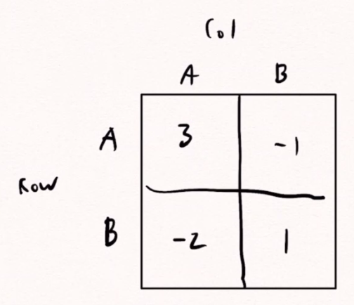
A strategy generally entails assigning a probability to choosing one particular row and column (either A or B in the above image). In the matrix, a numerical element represents the payoff for making that move.

The total payoff can be calculated as a weighted sum, where the payoff of a particular row or column is multiplied by the probability that it is chosen.

This can be converted into a linear program:

We must optimize max(min(col A, col B)), which is equivalent to min(max(row A, row B)) by strong duality.

This poses a problem though - taking the max of a min (or vice versa) is not a linear program! To fix this, we introduce a new variable $z$, and define constraints of z <= col A and z <= col B.

We can then formally define the problem:

• Objective function: max(z)
• Constraints on z: $M_{1,1}(p_1) + \cdots + M_{n,1}(p_n) \ge z$, and so on for each column in the matrix from $1$ to $m$. (The matrix $M$ is $n \times m$.)
• Constraints on the probabilities: $p_1 + p_2 + \cdots + pn = 1$ and $p_1, p_2, \cdots, p_n \ge 0$

Example (discussion 9) #

Here’s the payoff matrix:

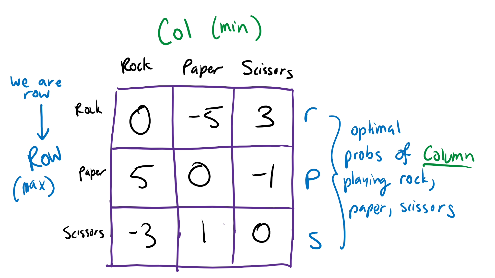
If Col. plays Rock, their payoff will be $0r + 5p - 3s$.

If Col. plays Paper, their payoff will be $-5r + 0p + 1s$.

If Col. plays Scissors, their payoff will be $3r - 1p + 0s$.

Objective: maximize $z$. (Maximize the minimum of column’s strategy, since Column should play optimally)

$z \le 5p - 3s$

$z \le -5r + s$

$z \le 3r - p$

$r, p, s \ge 0$

$r + p + s = 1$

The Experts Problem #

Suppose we have $n$ experts who each make a prediction (an integer) once per day. According to some rule, we will select one expert per day and follow their advice, which incurs a loss $f_{i(t)}^t \in [0,1]$.

Goal: Minimize the total loss $\sum_{t=1}^T f_{i(t)}^t$. (The loss is not revealed until after advice is chosen).

• One problem is the issue of the adversarial, an “expert” who intentionally wants to incur the highest loss possible. How do we avoid these adversarials even though we don’t know who they are?

Regret #

We cannot expect to always achieve smallest total loss. As such, we can redefine the problem to minimize regret, the expected value of the total loss given the selections in the previous days.

$R = \mathbb{E} [ \sum_{t=1}^T f_{i(t)}^t ] - (\min_{i \in [n]}\sum_{t=1}^T f_i^t)$

In other words, we pick the best expert in hindsight, such that we minimize the difference between the expected loss and actual loss for that day.

This reveals the selection strategy as follows:

• For each day $t$, set loss 0 for the expert with the lowest probability of loss on day $t$, and set loss 1 for all other experts.

Some strategies to pick experts #

Always pick the first expert: this is bad if the first expert is always wrong (loss 1), and another expert is always right (loss 0). This creates a regret of $R = T - 0 = T$.

Choose the majority opinion: if a singular expert is always right and the majority is always wrong, then the regret is still $R=T$.

Pick expert at random: Now, the regret is the difference between the average total loss and the minimum total loss.

$\sum_{i=1}^n 1/n \cdot F_i - \min F_i \le (n-1)/n \cdot T$ if we choose the best case for the first day, then the worst case for all of the other days.

Pick best expert so far: Since this is deterministic, it is still possible for the selected expert to always be wrong and everyone else to be right.

A better strategy (Weighted Majority) #

Binary version:

Fix a parameter $\epsilon$. Then, initialize weights $w_1^0 , \cdots, w_n^0$ to $1$ for all $n$ experts.

At time $t$, update each weight $w_i^{t+1}$ to be equal to $w_i^t$ if the expert was correct (loss 0), and $w_i^t \cdot (1-\epsilon)$ if the expert was wrong.

To make a decision, split the group into two, one which predicts A and the other which predicts B. One of the groups will be right, and the other wrong.

To choose between A and B, select the one whose experts have the higher weighted sum.

This strategy achieves $E \le 2(1+ \epsilon) (\min f_i^t) + \frac{2 \ln(n)}{\epsilon}$.

Multiplicative weight updates:

To improve on the above algorithm, rather than splitting experts into two groups (since fractional losses don’t support this), we choose an expert at random with probability $p_i^t = \frac{w_i^t}{\sum_{j=1}^n w_j^t}$ (the weight of this expert out of the sum of weights of all experts).

We then update only the expert that was chosen, with the rule $w_i^{t+1} = w_i \cdot (1- \epsilon f_i^t)$.

The expected value of this strategy is at most $\epsilon \cdot T + \frac{\ln(n)}{\epsilon}$.