Visibility and Shading

Overview #

Here’s the main steps for rasterizing an image:

• position objects in the world using transforms
• compute the position of objects relative to the camera
• project objects onto the screen
• sample and interpolate triangles using barycentric coordinates
• add texture maps
• disable objects that are not visible to the camera
• add shading

Visibility #

Objects can overlap others, such that some will not be visible to the viewer.

The Painter’s Algorithm is inspired by the process of painting an image: if you paint back to front, the images in the foreground will hide the background behind it.

• In practice, this requires sorting objects by depth (n log n problem). As such, it is not typically used.

The Z-buffer algorithm is a more optimized algorithm that stores the current min z-value for each sample position using a buffer. This algorithm is $O(N)$ with repsect to the number of triangles.

for T in triangles:
	for (x, y, z) in samples(T):
		if z < zbuffer[x, y]:
			framebuffer[x,y] = color[x,y,z]
			zbuffer[x,y] = z
		# else do nothing

• This can still be inefficient if you get unlucky and/or objects are sorted in reverse order. One mitigation for this is to do an approximate sort before Z-buffer.
• Another issue is transparency (drawing a transparent object in between two existing objects will not work). A common solution is to draw all opaque polygons first, then draw transparent polygons in sorted order.
  • Another solution is to store a linked list of transparent objects, and insert objects into the list when needed before rendering.

Shading #

The last component of rasterizing is to light objects.

Local shading #

Main idea: compute the amount of light reflected toward the camera

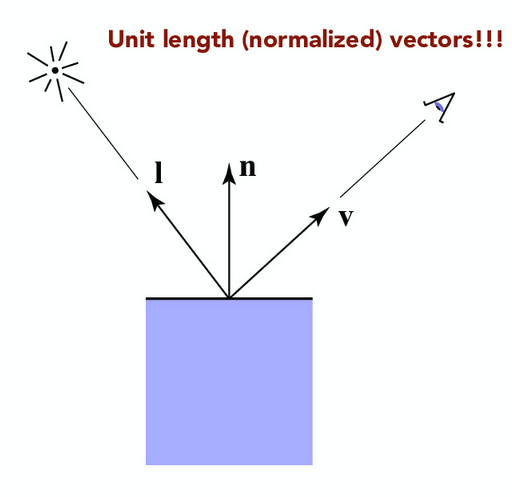
• $l$: direction of light
• $n$: normal vector
• $v$: direction of camera

By Lambert’s cosine law, the light per unit area is proportional to $l \cdot n$, which is equal to $\cos \theta$ assuming all vectors are normalized (where $\theta$ is the angle between $l$ and $n$).

Falloff: Light intensity decreases by distance based on $1/r^2$. This formula is used for global shading. However, for local shading, we approximate intensity using $1/r$, since we often want a more gradual dropoff in order to better light far-away objects.

Diffuse Shading #

Diffuse Lighting: Also known as Lambertian shading. Creates a matte appearance

• $L_d$ = diffusely reflected light
• $k_d$ = diffuse coefficient (rgb value)
• $I$ = illumination (strength of light)
• $r$ = distance from light
• $l \cdot n$: shading effect due to Lambert’s law
• In practice, this is a vector operation (do it once for each RGB color channel).

Specular Shading #

Specular Lighting creates a shiny appearance.

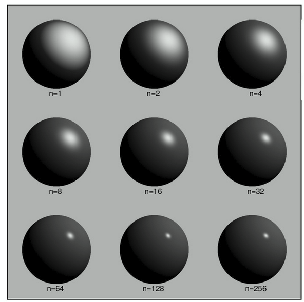
• Let $h$ be the half-angle vector between $l$ and $v$, computed using $$h = \frac{v+l}{||v+l||}$$ Then, we can compute the specularly reflected light using the formula $$L_s = k_s (I/r^2) \max(0, n \cdot h)^p$$
• $k_s$ is the specular coefficient (rgb value)
• $p$ is the power (larger $p$ = narrower, brighter lobe; smaller $p$ = wider lobe). A theoretically perfect mirror would have $p = \infty$. $p$ can be varied using a texture map.
• .

Point vs Direction lighting #

A point light exists in world space. As you move around the surface of an object, the relative location of the light changes.

A directional light is modeled to be infinitely far away (example: the sun). In this case, the direction of $l$ is constant, and equal to the negated direction of the light.

Ambient lighting #

Ambient lighting is constant, and does not depend on anything.

Overall lighting #

If we add the ambient, diffuse, and specular lighting values, we get the total illumination under the Blinn-Phong Reflection Model.

BRDF #

BRDF stands for “Bidirectional Reflectance Distribution Function.”

A BRDF takes: surface material, light direction, viewer direction, and orientation of surface; and outputs a color value. BRDFs can get complex, and are used to model real-life materials/mechanics (such as paints, subsurface scattering…)

Shading Frequency #

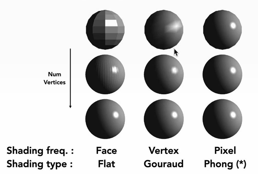
There are three main ways we can shade an object:

• Shade each triangle (flat shading): calculate one normal vector per triangle. This is not good for smooth surfaces.
• Shade each vertex (Gouraud shading): interpolate colors from vertices of triangles, where each vertex has a normal vector.
• Shade each pixel (Phuong shading): interpolate normal vectors across each triangle. This is more costly.

Calculating Vertex Normals #

Getting a surface normal of a triangle is fairly straightforward (just take the cross product of two edges).

Vertex normals are slightly more complicated, since vertices technically don’t have normal vectors. A basic strategy we could use is to take the average of the surrounding face normals.

To get per-pixel normals, we can use interpolation on vertex normals.

To transform a normal vector, use the inverse transpose of the transform matrix.