SQL Basics
Relevant Materials #
What is SQL? #
Structured Query Language (/ˈsiːkwəl/) is a highly standardized syntax for performing operations on a database.
Terminology #
SQL databases are a set of named relations, or tables, that describe the relationship between attributes. You can think of attributes as the columns of the table, and each record (also known as a tuple) being one row in the table.
Relations are composed of:
- A schema, which is the description of the table. Schemas are fixed, with unique attribute names and atomic types (integer, text, etc.).
- The instance, which is the set of data that satisfy the schema. Instances can frequently change (whenever a row is added or updated), as long as any additions are consistent with the schema.
As an example for using this terminology: if we add a column to the table, we can say that “we updated the schema of the relation to include an additional attribute”.
A note on looking up SQL things online #
The SQL syntax and features we cover in this course are known as “standard SQL”, whose specifications can be found here.
In the wild, there are many implementations of SQL (like SQLite, MySQL, MariaDB), which may have an extended feature set or slightly different syntax. We will generally stay away from these extended features, and you do not need to know them for now.
If you’re struggling to find relevant information, I would recommend prepending “sqlite” to the front of your search query (e.g. “sqlite how to create a table”). We use SQLite in Project 1, and for most things it’s safe to assume that the syntax will be what we’re looking for. Read more about SQL vs SQLite here.
Running SQL queries #
You will install sqlite3 in
Project 1. Once you’ve installed it, you can run sqlite3 in your terminal to start an interactive session, or run sqlite3 database.db to read from a file named database.db. Once in the session, you can also run .read file.sql to run queries written in the file file.sql, or run .schema to get schema information for the current database.
In a pinch, the CS61A online interpreter also works great, and has a built-in visualizer that’s especially useful for exploring aggregation.
Pedagogy note #
Don’t get too hung up on the syntax, or remembering how to use every small feature of SQL. The language itself is only a small part of this course- for most of our time, we’ll discuss how to actually implement the features you use here.
If you anticipate needing SQL in future work, here’s a nice reference for common keywords and how to use them.
Keys #
When defining schemas, it’s often important to be able to guarantee that rows are unique so that we can catch duplicate information. For example, if the school had a database of all enrolled students, we wouldn’t want two students to have the same SID!
Primary Keys #
Primary keys are unique, non-null, and can be used to identify an entry. Many times, adding PRIMARY KEY (id) during
table creation is good enough.
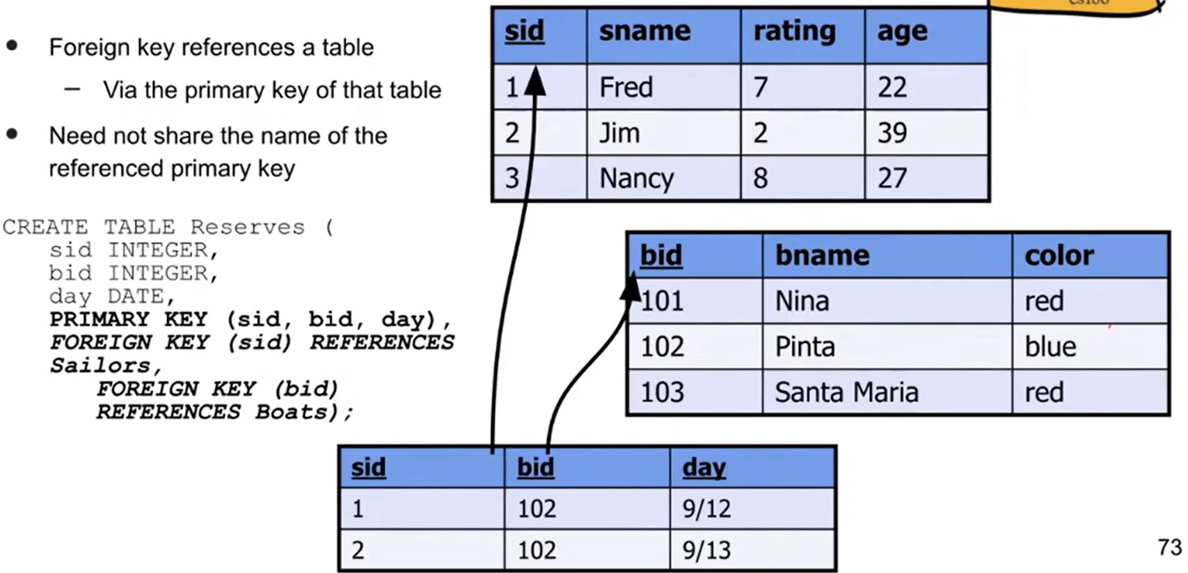
In other cases, like the boat reservation tracking example in lecture, we would need more than one attribute (PRIMARY KEY (sid, bid, day)) to guarantee uniqueness, since a boat can be reserved many different times.
Foreign Keys #
Foreign keys reference other tables’ primary keys. Building onto the boat example, the boat ID would be the same as the ID’s in a table of boats, so we could add FOREIGN KEY (bid) REFERENCES Boats to the reserves table instead of copying everything over.
The main purpose of foreign keys is to maintain the uniqueness and non-null constraint of an attribute, since it has to match the primary key of another table.
Below is a screenshot from lecture that puts some code to the example.
Writing Queries #
Enough with the long complicated words, let’s write some SQL!
Create Table #
First, let’s create a table:
CREATE TABLE clubs(
	name TEXT,
	alias TEXT,
	members INTEGER,
	PRIMARY KEY (name)
) AS
SELECT "Computer Science Mentors", "CSM", 500 UNION
SELECT "Open Computing Facility", "OCF", 50;
Here’s a good list of common data types that you can use. For the purposes of this class we will mostly focus on INT, BOOLEAN, TEXT, CHAR(n), VARCHAR(n), and BYTE. More about what these do in the next section.
Insert Values #
There’s more clubs to add! Let’s add one after the table has already been created:
INSERT INTO clubs VALUES
	("Eta Kappa Nu", "HKN", 100),
	("Computer Science Association", "CSUA", 200);
Basic Querying #
Below is the basic structure of a query:
SELECT name AS clubname
FROM clubs
WHERE members >= 100 AND members <= 300
ORDER BY clubname
LIMIT 3;
Here, we:
- SELECT the column
nameFROM the tableclubs, and rename it toclubname; - Keep only the clubs WHERE the number of members is between 100 and 300;
- Sort the entries by name (ascending by default),
- and keep only the top 3 entries (by alphabetical order).
Aggregation #
Aggregation can seem tricky, but the core idea is simple: crunch similar rows into one row, and keep one particularly interersting value.
There are three parts to this:
- GROUP BY: Specify the column containing the similar values. All rows with the same value in this column will be combined into one row.
- HAVING: Specify how you want to filter (this is optional.) The syntax is basically the same as
WHERE, except instead of a column name, we use an aggregate on a column name (such asMAX(members)orCOUNT(*)). - Modifications to SELECT: Ensure that all of the selected columns (except the one(s) passed into GROUP BY) are aggregates (MAX, MIN, COUNT, SUM…).
It’s possible to GROUP BY multiple columns. This will group together every combination of values in those two columns. For example, if we did GROUP BY name, alias, and two clubs Open Computing Facility and Original Cat Friends had the same alias OCF, they would represent two separate groups.
WHERE and HAVING?In short, WHERE operates on individual rows, and HAVING operates on groups.
Whenever you want to do something that requires the GROUP BY to have been done first, like filter by MAX(members) > 100, it needs to be in the HAVING clause.
Practice Problems #
Still unsure about querying and aggregation? Here are some of my old 61A discussion slides that have some practice problems (back when we still taught SQL). All of the tables referenced are already preloaded for you in code.cs61a.org.
Logical Processing Order #
SQL Queries are typically processed in a different order than they’re written. Here’s the order- try to develop an intuition as to why this order would make more sense to a machine than how queries are usually written:
FROM(find the table that is being referenced, join if needed)WHERE(filters out rows)GROUP BY(aggregate)HAVING(filters out groups)SELECT(choose columns)ORDER BY(sort)LIMIT(cut off the output)
When writing queries, I often like to follow this order as well since each step builds on the previous one.
A note on aliasing #
One consequence of Logical Processing Order is that we cannot use aliases in WHERE, GROUP BY, or HAVING because they are processed before any alias is defined in SELECT!
For example, SELECT name as clubname WHERE clubname = 'Open Computing Facility' is NOT a valid query in standard SQL.
However, since ORDER BY and LIMIT come afterwards, we are allowed to use aliases there.
Joins #
 If we have two tables and need to access information from both in a query, we will need to join the two tables together!
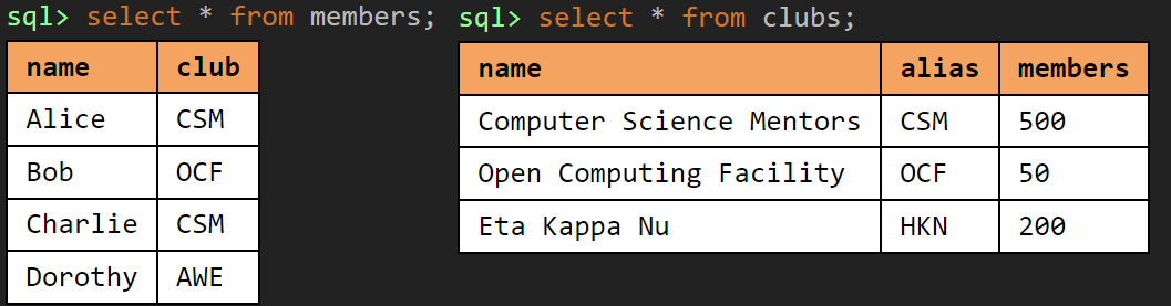
For this section, we will use the following tables as examples:
Cartesian Product #
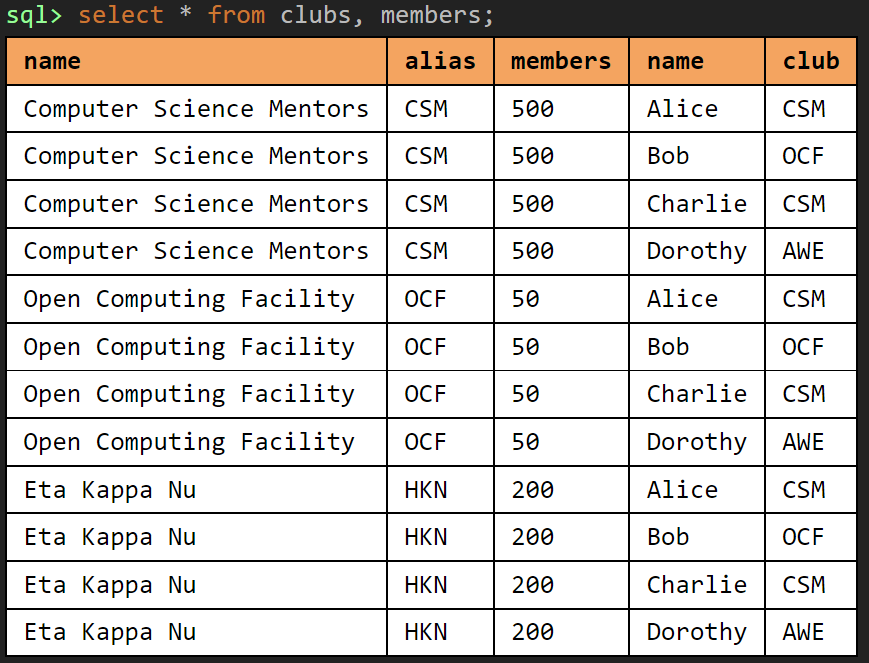
By default, if a join (SELECT ... FROM a, b...) is done in SQL without specifying a type, a cross product (Cartesian product) is calculated. Every row in table a (the left table) is combined with every row in table b to create $R_a * R_b$ rows ($R_a$ = number of rows in table a).
In the example below, since clubs had $2$ rows and members had $4$ rows, we should expect the result to have $3 \times 4 = 12$ rows. Note that most of these rows are pretty useless, since there is no correlation between the member and the club they were joined with.
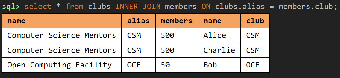
Inner Join #
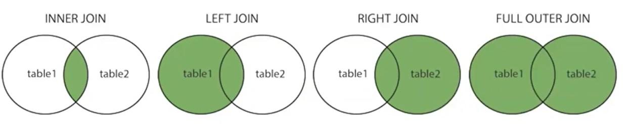
An inner join takes only the rows in which a particular attribute (or list of attributes) can be found in both the left and right tables.
For example, an inner join on the
sidattribute could be written out asSELECT ... FROM a, b WHERE a.sid = b.sid.Inner join is the default behavior for the JOIN operation, which looks like this:
SELECT ...
FROM a INNER JOIN b
ON a.sid = b.sid
...
In the example below, we only keep the clubs CSM and OCF, and only keep the members that are in those two clubs:
Natural Join #
A NATURAL JOIN automatically inner joins tables on whichever attributes share the same name between the two tables.
If the columns alias and club were both named the same thing, then SELECT ... FROM a NATURAL JOIN b ... is completely equivalent to the example in the inner join section above. Otherwise, the NATURAL JOIN will return an empty table if no column names are shared (even if the contents are the same).
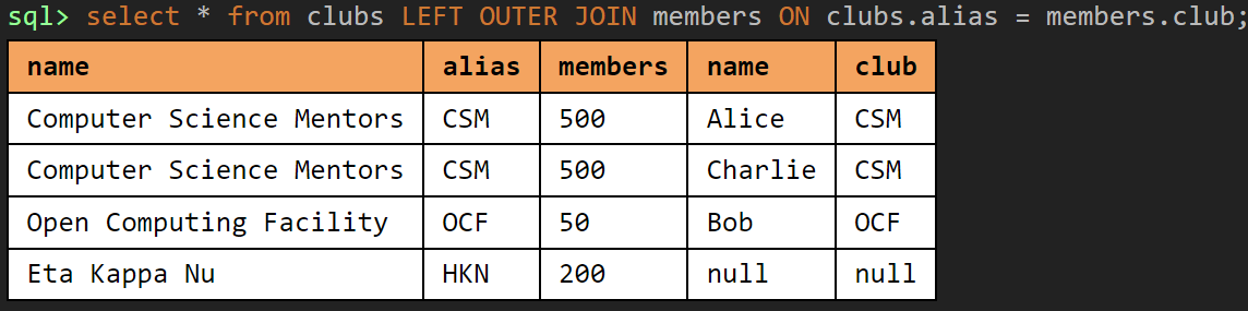
Outer Join #
Left outer joins return all matched rows (as in an inner join), AND additionally preserves all unmatched rows from the left table. Any non-matching fields will be filled in with null values.
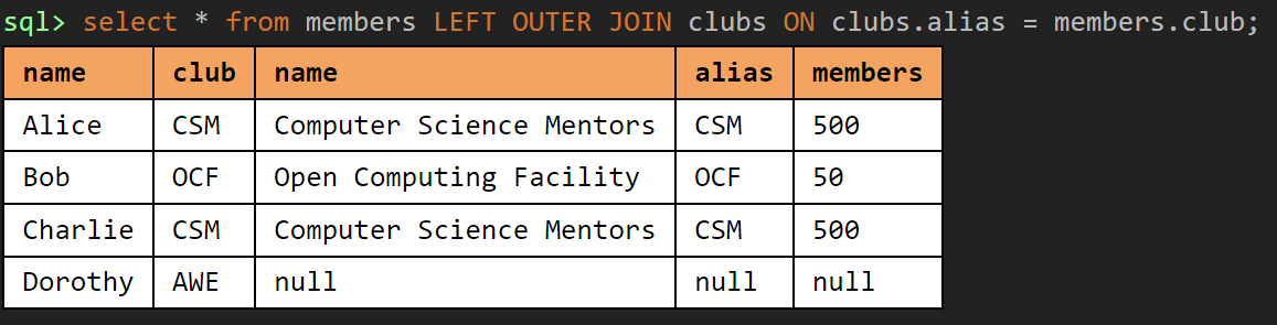
A right outer join is the same as the left outer join, except it preserves unmatched rows from the right table instead. Flipping the table order on a left outer join creates an equivalent right outer join:
A full outer join returns all rows, matched or unmatched, from the tables on both sides of the join clause.
Advanced Mechanics #
String Comparisons #
Using the LIKE operator, we can do the following:
- Match any single character:
_ - Match zero, one. or multiple characters:
% - Example:
WHERE name LIKE 'B_%'will match all rows with a name starting with a B and are at least 2 characters long
Unions and Intersections #
The UNION operator combines two queries (like an OR statement).
The INTERSECT operator combines two queries, and discards rows that do not appear in both (like an AND statement).
The EXCEPT operator subtracts one query’s results from another.
UNION, INTERSECT, and EXCEPT operate using set semantics (distinct elements) and will keep only one of each unique element in the result.
Using UNION ALL, INTERSECT ALL, and EXCEPT ALL will manage cardinalities and will add or subtract the number of identical elements accordingly.
- UNION ALL = sum of cardinalities
- INTERSECT ALL = minimum of cardinalities
- EXCEPT ALL = difference of cardinalities
Nested Queries #
The IN operator allows subqueries to be made. For example, we can SELECT ... FROM ... WHERE id IN (SELECT .....)
- The
EXISTSkeyword can be used in place ofINto make correlated subqueries where the table in the subquery interacts with the outer query. ANYandALLcan be used as well:SELECT * FROM a WHERE a.value > ANY (subquery...)would only keep rows inathat are bigger than the smallest value in the subquery.ALLcan be used to compute an argmax: for example, if we want a sailor with the highest rating, we canSELECT * FROM s WHERE s.rating >= ALL(SELECT s2.rating FROM s s2)
Views #
A view is a named query. It can be thought of as a temporary table that can be accessed in future queries to make development simpler. Unlike tables, it is not computed immediately, and results are cached when they are needed.
CREATE VIEW name
AS SELECT ...
A “view on the fly” can also be created using the WITH keyword:
WITH name(col1, col2) AS
(SELECT ...),
name2(col1, col2) AS (SELECT ...),
SELECT ...