Bayes Nets

Probability Review #

For the underlying probability theory (independence, conditional probability, distributions), see probability-overview. For Bayesian parameter estimation on the resulting CPTs, see parameter estimation.

Bayes Nets #

Bayes Nets consist of:

• Nodes corresponding to a variable in the problem
• A CPT (Conditional Probability Table) for each node
• Edges between variables that encode a direct influence (conditional probability)

Properties:

• Must be a directed acyclic graph (no cycles)
• Space complexity: $O(n \cdot d^k)$
  • $n$ variables (number of CPT’s)
  • $d$ possible values per tables
  • $k$ maximum variables in one table

Global semantics:

• Must have exactly one probability term per node: for all nodes $X$, global semantics must include $P(X|\cdots)$

Independence in Bayes Nets:

• Write out chain rule to relate variables: $P(X_1, X_2, \cdots, X_n) = \prod_{i=1}^n P(X_i | X_{i-1}, X_{i-2}, \cdots, X_1)$
  • Example: $P(A, B, C) = P(A|B,C)P(B|C)P(C)$
• Compare Bayes net global semantics to chain rule, and all terms that do not match suggest (conditional) independence
• Every variable is conditionally independent of ancestors (parents’ parents, etc), given parents
• Every variable is conditionally independent of all other variables given Markov blanket (children, parents, and children’s parents).

Inference by Enumeration #

Any probability can be computed by summing up entries from the joint distribution: for example, $P(Q|e) = \sum_h P(Q, h, e)$.

If we do this repeatedly on a Bayes net expansion, we can essentially get the probability of any variable(s) conditioned on any other variable(s). This method is called inference by enumeration.

Variable Elimination #

Variable elimination is an algorithm that attempts to intelligently choose the order of summations to minimize the number of operations that need to be completed.

The core element of variable elimination is factors, which represent multidimensional distributions of a set of variables. The primary difference between factors and probabilities is that factors do not necessarily sum up to 1 over all possible values.

In order to convert factors back to probabilities, they need to be normalized by applying the definition of conditional probability (dividing the factor by the sum of probabilities for all possible values of the queried variable).

Important note: By convention, uppercase variables are random variables themselves; lowercase variables represent specific values of those variables.

Here’s an example of variable elimination in action. Consider the following Bayes Net:

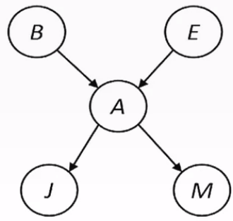
This can be represented as the equality

Let’s suppose we are trying to find $P(B|j,m)$. This means that we need to eliminate the variables $A$ and $E$:

$P(B|j,m) = \sum_{e, a} P(B, e, a, j, m) = \sum_{e, a} P(B) P(e) P(a|B,e) P(j|a)P(m|a)$

First, we move summations inwards as far as possible:

$P(B) \sum_e P(e) \sum_a P(a|B,e) P(j|a) P(m|a)$

Next, we can create factors for each of the summations.

• $$f_1(B, e, j, m) =$$

Sampling #

In practice, getting the exact probability of an inference is not required as long as we get a rough estimate (80% chance is basically the same as 80.15%, etc.).

In order to cut down on the resources required to make inferences from a Bayes Net, we can use sampling techniques to approximate the true probability of a query.

Prior Sampling #

For all $i$ in topological order , sample $X_i$ from the CPT of $P(X_i | parents(X_i))$.

Then, return the tuple of all $x_i$ sampled.

The probability of getting an exact tuple $(S(x_1, \cdots, x_n)$ is equal to $P(x_1, \cdots, x_n)$ from the original Bayes Net.

As the number of samples taken gets larger, the number of samples that equal a particular tuple divided by the total number of samples approaches the true probability. This means that prior sampling is consistent.

Rejection Sampling #

If we’re trying to evaluate a particular query $P(Q | e)$ using prior sampling, it’s possible that the vast majority of samples taken don’t actually reflect the conditional we want (i.e. $e$ is a different value from desired).

We can save on computation by immediately rejecting all samples that don’t match the query, and not fully calculating their probabilities.

Likelihood Weighting #

Now, one issue that arises from rejection sampling is that if the evidence is unlikely, then we will have to reject lots of samples and the total number of relevant samples will be very low. This is common in real-world problems where variable domain sizes can be massive (millions or billions of possible value).

Main idea: assign weights to each sample corresponding to their likelihood of matching the query. When adding up samples, multiply them by their weight.

Mathematical representation:

$S(z,e) \cdot w(z,e) = \prod_j P(z_j | parents(Z_j)) \prod_k P(e_k | parents(E_k)) = P(z, e)$

• For example, if estimating $P(-a | +b, -d)$, then the sample -a +b +c -d would have a weight equal to $P(+b|-a)P(-d|+c)$.
• Pseudocode:

weight = 1.0
sample = []
for every variable X:
	if X is an evidence variable:
		add X to sample
		weight *= P(X | parents)
	else:
		sample X from P(X | parents) using random number generator
		add X to sample

• To estimate the probability using likelihood sampling: $P(q | E)$ = sum of weights of samples that match query+evidence divided by sum of weights of all samples that match evidence

Gibbs Sampling #

A particular kind of Markov Chain Monte Carlo:

• A state is a complete assignment to all variables.
• To generate the next state, pick a variable and sample a value for it conditioned on the other variables.
• $P(X_i | x_1, \cdots, x_{i-1}, x_{i+1}, \cdots)= P(X_i | markov\_blanket(X_i))$