Markov Models

A Markov Model is basically a Bayes net that is an infinitely long chain (”time series bayes net”).

Typically, each node is a random variable that represents a specific point in time.

Markov models follow the memoryless property, which states that the random variable for time step $i+1$ is independent of all other variables except the random variable at time step $i$. (For the probability-theory foundation of this construction, see markov-chains.)

Additionally, Markov Models are stationary: for all values of $i$, $P(S_{i+1}|S_i)$ are all the same. This means that a Markov Model can be represented with only two CPT’s: one for $P(S_0)$ and one for everything else.

The joint probability represented by a Markov Model can be written as follows:

Mini-Forward Algorithm #

By the chain rule, $P(W_{i+1}) = \sum_{w_i} P(W_{i+1} | w_i)P(w_i)$.

• For every timestep $i$, we compute the probability of all possible values $w_i$ given all previous values, then advance the model by one timestep to get the and use the previously calculated values as the new CPT.

Stationary Distribution #

The stationary distribution is the conditional probability values that the Markov model converges to as time increases unboundedly ($W_\infty$).

In order to get this distribution, we must use the mini-forward algorithm on all possible values of $W_{i+1}$, then combine them into a system of equations to solve.

Hidden Markov Models (HMM) #

In addition to the state variables that regular Markov models have, Hidden Markov models introduce evidence variables that represent new findings at each timestep that could alter the distribution for just that timestep.

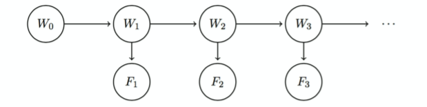
• All evidence variables $F_i$ are conditionally independent to all state variables given $W_i$.
• All state variables are conditionally independent to all state and evidence variables given $W_{i-1}$.
• $F_1$ is conditionally independent to $W_0$ given $W_1$.

In HMMs, the sensor model $P(F_i|W_i)$ is stationary (i.e. the same for all values of $i$). This means that any HMM can be represented with three CPT’s: the initial distribution, transition model, and sensor model.

The belief distribution at time $i$ describes the current state given all of the evidence that we know so far: $P(W_i|f_1, \cdots, f_i)$

Forward Algorithm #

$B(S_t) = P(S_t | \textnormal{all evidence up to t)} = P(S_t|e_{0:t}) = \frac{P(e_t | S_t)P(S_t | e_{0:t-1})}{P(e_t|e_{0:t-1})}$

• Time elapse: $B’(S_{t+1}) = \sum_{s_t} P(s_{t+1}|s_t)B(s_t)$
• Observation update: $B(S_{t+1}) = \alpha \times P(e_{t+1} | s_{t+1}) B’(s_{t+1})$
  • Need to normalize by probability of evidence given past evidence.

Using Bayes’ Rule:

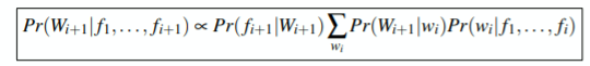
1. Time elapse update: determine $B'(W_{t+1}|f_1,\cdots,f_{t+1}) = \sum_{w_t} P(w_{t+1} | w_t)B(w_t)$
2. Observation update: using the time elapse update, determine $B(W_{t+1}) =P(W_{t+1}|f_1, \cdots, f_{t+1}) = \alpha P(f_t | W_{t+1})P(W_{t+1}) = P(f_t|W_{t+1})B'(W_{t+1})$
3. Normalize by dividing the observation update value by the sum of entries in the probability table for $P(W_t | f_t)$ (i.e. probability of evidence given past evidence)

Particle Filtering #

Particle filtering is the Bayes Net sampling equivalent for Hidden Markov Models: when it becomes too expensive to do exact inference, we can instead approximate the probability distribution. (For more on the underlying sampling techniques, see sampling.)

Here’s how the simulation goes:

• Start with $n$ particles, which are each at one of the $d$ possible states. Typically $n$ is much smaller than $d$.
• Perform a time elapse update: for every particle at state $t_i$, sample the updated value from the CPT of $P(T_{i+1}|t_i)$ (using RNG).
• Perform an observation update: for a particle in state $t_i$ with sensor reading $f_i$, assign a weight of $P(f_i|t_i$).
  • Calculate each individual weight, then calculate the total weight for each state.
  • If the sum of all weights is 0, reinitialize all particles.
  • Otherwise, normalize the distribution of weights and resample the particles from this distribution. Never resample if there is no evidence because it will just introduce more (possibly detrimental) randomness.