Neural Networks

General idea: Combine multiple simple regression models together to increase complexity of the overall model.

Optimization #

Gradient Ascent and Descent #

The difference: gradient ascent maximizes a log-likelihood function; gradient descent minimizes a loss function.

Gradient Ascent algorithm:

randomly init w
while w not converged:
	for weight in w:
		weight = weight + learning_rate * gradient(log_likelihood(w), weight)

• convergence is when gradient = 0, or no change occurs between two runs
• $w$ is a vector of $N$ weights
• gradient(log_liklihood(w), weight) represents the operation $\nabla_{weight} \log l(\bold{w})$, which returns a vector of $N$ partial derivatives $\partial_{weight} \log l(w_i)$ for every weight $w_i$.

Gradient Descent algorithm:

randomly init w
while w not converged:
	for weight in w:
		weight = weight - learning_rate * gradient(loss(y, x, w), weight)

• Basically the same as gradient ascent, except subtract the gradient of loss instead of adding the gradient of log likelihood.

Stochastic gradient ascent/descent: only take one data point at a time to calculate the gradient. May cause inaccurate results.

Batch gradient ascent/descent: Randomly takes a batch size of $m$ data points each time to compute the gradients. Good compromise in terms of performance and accuracy.

Multilayer Perceptron #

Main idea: make perceptrons take outputs from other perceptrons as their input.

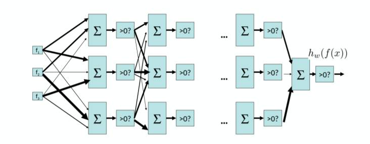
Universal functional approximator theorem: a two-layer neural network with enough neurons can approximate any continuous function to any desired accuracy.

In order to approximate nonlinear functions, each layer is separated by a nonlinear operator. Traditional neural nets have used the sigmoid function $\sigma(x) = \frac{1}{1 + e^{-w^Tx}}$, but due to faster computation the ReLU (rectified linear unit) function is often used instead. The graphs of these two functions are as follows:

For every layer, we wrap the parameters around a function call. For example, here is a 2-layer network:

• $x$ is an $1 \times i$ input vector
• $W_1$ and $W_2$ are $i \times h$ weight parameter matrices, where $h$ is the hidden layer size parameter
• $b_1$ and $b_2$ are $1 \times h$ bias parameter vectors