 ben's notes
Search Problems
Search problems consist of:
- A state space $S$
- An initial state $s_0$
- Possible actions $A(s)$ in each state
- Transition model that converts a current state and action into the next state
- A goal test $G(s)$ that returns true or false depending on if $s$ is at the goal
- An action cost
As an example, suppose you are travelling:
- The state space is all cities you can go to.
- The initial state is which city you start in.
- Actions are to navigate to adjacent cities.
- The transition model is the process of travelling to another city.
- The goal test is to check if you are in the desired city.
- The action cost is the road distance.
Search problems are typically conducted on models, which are imperfect representations of the real world. Models are almost always wrong to some extent.
A search is complete if a solution is guaranteed to be able to be found.
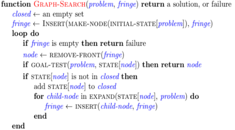
- Tree searches may not be complete if an infinite loop exists.
A search is optimal if the solution found is guaranteed to be the shortest path.
State spaces can be represented with a state space graph, where nodes are possible configurations (states) and edges represent actions (transitions). In a state space graph, each state occurs only once - this is in contrast with search trees, where states can appear in multiple paths.
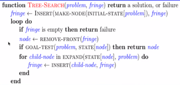
Solving Search Problems #
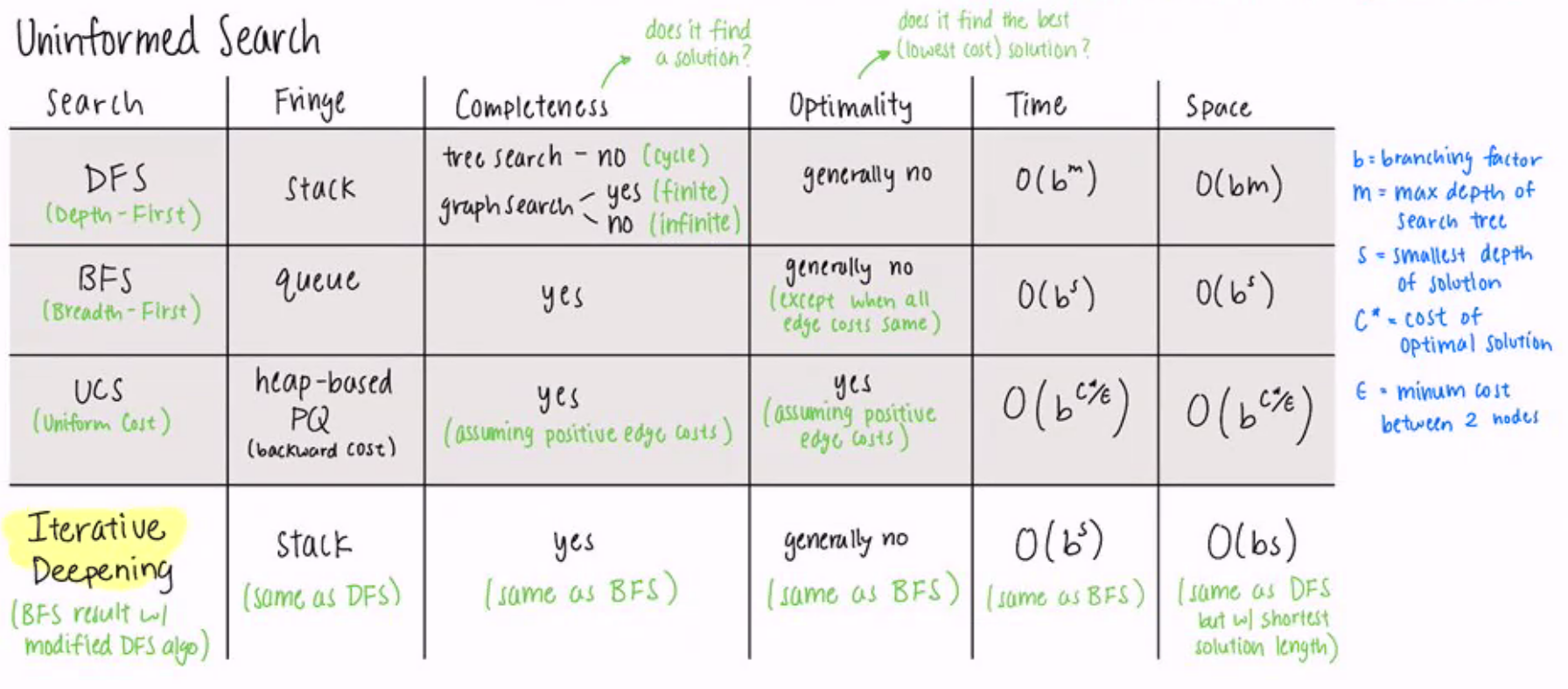
BFS: queue (see breadth-first-search-bfs for an introductory walkthrough, and Graphs for the runtime analysis)
- Takes $O(b^s)$ time where $s$ is the depth of the shallowest solution
- Takes $O(b^s)$ space since the entire bottom tier needs to be loaded
- Is complete (if a solution exists, then $s$ must be finite), but not optimal (if the costs are not equal)
DFS: stack (expand deepest node first; see depth-first-search-dfs)
- Takes linear space (only one path in memory at a time)
- But can take exponential time $O(b^m)$ where $b$ is branching factor and $m$ is depth
- Not complete (if $m$ is infinite) or optimal (if the leftmost infinite branch is only explored)
Iterative Deepening: combine DFS space advantage with BFS time advantage
- Run DFS with depth limit $n$, where $n$ starts at $1$ and increments if no solution is found
Uniform Cost Search (Dijkstra’s but don’t initialize distances): Priority Queue or heapq
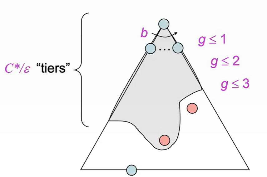
- Expands the path with the lowest $g(n)$, where $g(n)$ is the cost to go from root to $n$
- Takes $O(b^{C^*/\epsilon})$ time, where the solution costs $C^*$ and the smallest arc is $\epsilon$
- Also takes $O(b^{C^*/\epsilon})$ space (same logic as BFS)
- Both complete and optimal, assuming $C^*$ is finite and $\epsilon \gt 0$
- Basically A* with a null heuristic ($h(X) = 0 \\ \forall X$
Informed Search #
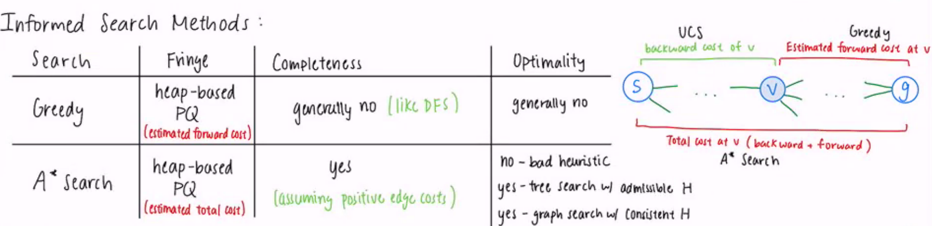
Searches can use heuristics to guide their direction. Heuristics are estimated costs to the goal (often solutions to simpler/relaxed problems).
A good heuristic must be:
- Admissible: (optimistic): ****positive and less than the true optimal forward cost to goal
- $0 \le h(v) \le h^*(v)$ for all $v \in V$
- In other words, it underestimates the cost to the goal
- Admissible heuristics are often solutions to relaxed problems (more available actions, like allowing Pacman to go through walls)
- Consistent:
- $h(u) - h(v) \le d(u, v)$ for all $(u, v) \in E$
- In other words, it underestimates the weight of every edge
Admissible heuristics are not necessarily consistent, but consistent heuristics must be admissible.
A heuristic $h_1$ is dominant over another heuristic $h_2$ if for all states $n$, $h_1(n) \ge h_2(n)$.
- In other words, larger is better as long as both heuristics are admissible.
- If there are two heuristics where neither dominates the other, we can create a dominant heuristic by taking the max of the two heuristics.
A* Search #
A* search is uniform cost search that expands the fringe node with the lowest heuristic value. (Expands a node $n$ such that the cost of the best solution through $n$ is optimal)
A* ends when the goal is dequeued, not when it is enqueued.
- A* tree search is optimal with an admissible heuristic.
- If there exists an optimal goal $A$ and suboptimal goal $B$, $A$ will always be expanded first in the tree because some ancestor $n$ of $A$ must be expanded before $B$.
- $f(n) = g(n) + h(n)$ and $h(n) \le h^*(n)$, so $f(n) \le g(A) = 0 + f(A)$
- Since $g(A) < g(B), f(A) < f(B)$.
- Since $f(n) < f(A)$ then $f(n) < f(B)$. Therefore, the path from $n$ to $A$ will always be chosen over the path to $B$ if the heuristic is admissible.
- If there exists an optimal goal $A$ and suboptimal goal $B$, $A$ will always be expanded first in the tree because some ancestor $n$ of $A$ must be expanded before $B$.
- A* graph search is optimal with a consistent heuristic.
Local Search #
In many optimization problems, the path is irrelevant and all we need to know is the goal state itself.
- Some examples: travelling salesperson, n-queens (placing n queens where they can’t attack each other)
Iterative improvement algorithms keep a single current state and try to improve it.
- The main benefit of this is that it takes constant space.
Hill Climbing #
A simple iterative idea:
- Start anywhere
- Move to the best neighboring state
- If no neighbors are better than the current state, then quit
- Use a heuristic to evaluate quality of state
Hill climbing is ineffective when there are local maximums or plateaus (flat local maximum).
One possible mitigation for local maximums is to conduct random restarts (choose a new random starting state, and re-run the algorithm). It is guaranteed to eventually find the global maximum if enough restarts are conducted.
Simulated Annealing #
As a solution to getting stuck at local maxima, we occasionally and randomly allow “bad” (suboptimal) moves based on a temperature schedule.
for t in range(1, inf):
	temp = schedule(t)
  if temp == 0:
		return current_state
	next_state = randomSuccessor(current_state)
  delta = next_state.value - current_state.value
	if delta > 0:
		current_state = next_state
	else:
		current_state = next_state if random_probability(e**(delta/temp))
Intuition:
- Over time, the probability of choosing a bad move approaches 0.
- This algorithm is guaranteed to converge to the global maximum if the temperature decreased slowly enough.
- Delta is a negative number if used to calculate probability (since this means the next state is worse). The worse the state is, the more negative delta will be, which makes the probability of a very bad state being chosen smaller than a slightly worse state.
Local Beam Search #
Make $K$ copies of a local search algorithm, initialized randomly.
For each iteration, generate all successors from the $K$ current states, and choose the best $K$ successors to be the new current states.
- This is different from $K$ independent searches because the searches are coordinated (best ones will be favored dynamically).
- This is similar to how natural selection works.
Genetic Algorithms #
To further explore the analogy to evolution, genetic algorithms:
- Resample $K$ individuals at each step, weighted by a fitness function.
- Combine the individuals using pairwise crossover operators.
- Occasionally, introduce random mutation.