Caching

The Problem #

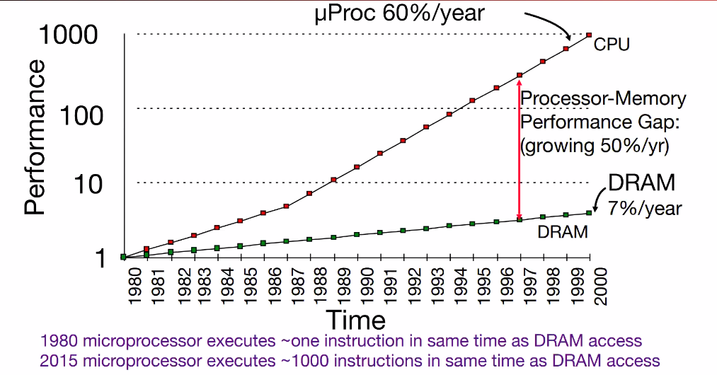
Over time, the processor-DRAM latency gap has been increasing, such that instructions relying on DRAM access greatly reduce the number of instructions that can be processed, and therefore the overall performance of a CPU.

A Solution: Caching #

Since programs only care about a very small subset of the total information available, if we identify this subset and place it into more local memory, then we can efficiently perform most memory accesses.

This process is called caching. The same principle reappears at higher levels of the system stack: see Chapter 8 Caching for caching in the OS (TLBs, page caches) and 03 Buffer Management for the database buffer pool, which is essentially a cache between disk and memory.

Caches give the benefits of speed from the fastest types of memory while still having the capacity of the largest memory. Ideally, caches are implemented such that they are invisible to programmers: they will automatically move memory between locations.

If we overwhelm the cache, though, performance will drastically decrease,

The Memory Hierarchy #

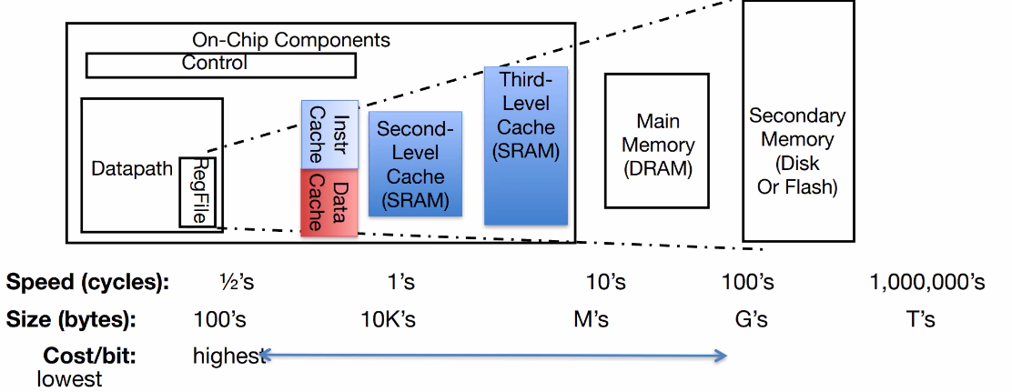
Smaller containers are generally faster to access, but more expensive to produce.

Cache level is the order of a particular cache in the level hierarchy: L1$ is closest to the processor, and is the smallest and fastest.

There is usually one L1 cache for instructions, and L2 cache is used for data.

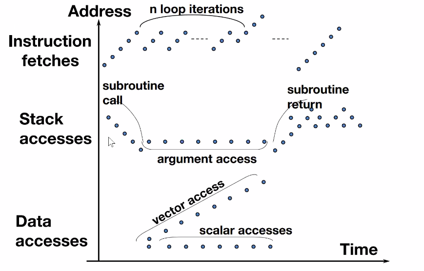
Locality #

There are two different types of locality:

Temporal Locality: locality in time. If a memory location is referenced, then chances are it might be needed again soon and so we should keep it around.

Spatial Locality: locality in space. If a memory location is referenced, then chances are the addresses close to that will be needed soon and should be saved to faster memory.

Here are some examples of patterns of locality:

Branch Prediction Locality #

Main Idea: If a branch is taken/not taken, then it is more likely than not that the next time the branch is evaluated, it will have the same result.

In other words, branches have temporal locality. If we save the result of the previous evaluation and load that into the cache,

This idea can work with:

• For loops (doing stuff until a condition is met - more likely to actually do the stuff rather than skip to the end)
• Rare conditionals (such as error checking)

Branch prediction can be done with a direct-mapped memory. When a new branch is fed into the branch comparator, the PC is set to the value in memory pre-emptively. When the branch is actually evaluated, we can determine if a kill is needed or not. The hope is that fewer kills are needed overall.

A similar idea with jal or jalr instructions is that we can keep a small stack of instructions located at PC+4 so that these can be immediately loaded when a function returns. We should always be able to correctly predict a function return address (as long as the stack is big enough).

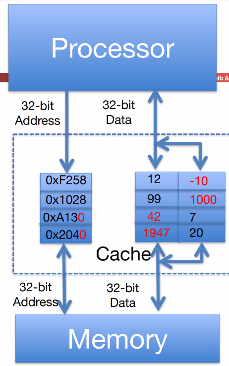
Memory Accessing with Cache #

Suppose we have a lw instruction.

1. First, the processor issues an address to the cache.
2. Then, the cache checks if the address has a copy of the data desired. If there is a match, then the cache sends the data to the processor. If not, then the cache sends the address to the memory, which then reads and sends the data to the cache to store.
3. The processor loads the value into the desired register.

Some Cache terminology #

A cache hit occurs when the memory address we’re looking for is actually stored in the cahce.

A cache miss is when we are looking for information that is in the main memory, but not the cache.

A valid bit is flipped if a particular entry is valid. If the valid bit is not on, then we should treat an access like a cache miss.

A cache flush invalidates all entries.

The cache capacity is the total number of bytes in the cache.

A cache line, other wise known as a cache block, is a single entry in the cache.

The block size is the number of bytes in each cache line/block.

We can calculate the number of cache lines by dividing the cache capacity by the block size.

Eviction is the process of removing an entry from the cache.

The Anatomy of a Cache #

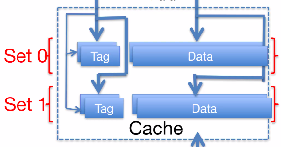
Caches have tags (addresses) and blocks (aligned words that store information).

In order to simplify the comparison process (so that we don’t need to check every tag to see if we have a hit or miss), we can split the cache into sets. So we only need to compare a tag to a particular set in order to determine if we have a hit or miss.

Types of Caches: Associativity #

Fully associative cache: Blocks can go anywhere. This is the most flexible option, but requires a large number of comparators (1 per block).

Direct mapped cache: Each block goes into one place, such that each set contains exactly one block. This makes it straightforward to check if a block exists (since there is only one place it can possibly go), but is the least flexible.

N-way Set Associative: There are N places for a block, such that each set has N number of blocks. This is a compromise between fully associative (N = # blocks) and direct mapped (N = 1).

Handling Stores with Write-Through #

When store instructions write to memory, we change the values. We need to then change both the cache value and the memory value to make sure that everything remains consistent.

We can use the write-through policy which states that we need to write values to both cache and memory. Since writing to memory is slow, we can instead write to a write buffer which stores the desired value until it is done being written.

The write-back policy states that we should write only to cache and then write the cache block back to memory when the block is evicted from the cache. That way, there is only a single write to memory per block, and writes are collected in the cache.

• Using the write-back policy, we include a “dirty” bit to indicate if a block was written to or not.

Write through vs. write back #

Write through is good because:

• It has simpler control logic.
• There is more predictable timng.
• It’s easier to make reliable since there is memory redundancy (both cache and DRAM have new values).

On the other hand, write-back:

• Is more complex, with variable timing.
• Reduces write traffic since we do fewer writes.
• Sometimes, only cache has data and so cache failure would result in disaster.

Write Allocate vs No Write Allocate #

If a cache write allocates, then if writing to memory not in the cache we should fetch it from memory first.

For no write allocate, we just write to memory without fetching.

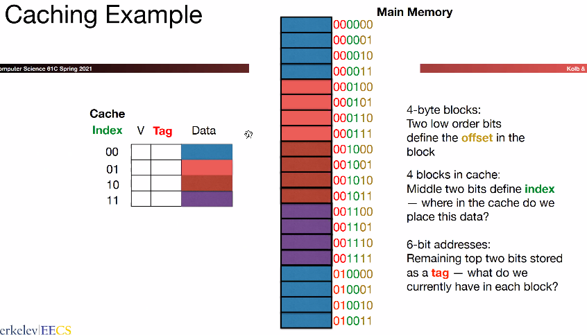
Tags, Index, Offset: The Address #

Addresses in the cache are divided into tag, index, and offset.

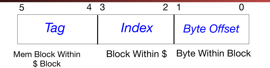
Offset #

Tells us where data exists in the cache line.

Contains $\log_2(blocksize)$ number of bytes (not bits) (for example, 64 byte blocks can be represented using 6 offset bits).

Index #

Tells us the where in the cache an address might be stored.

Contains $\log_2$(num cache lines / associativity) number of bits.

For example, a 4 way associative cache with 512 lines requires 7 index bits.

Tag #

Determines which memory location in the cache that the data is stored.

The number of bits in the tag is just the bits remaining (total address bits - index bits - offset bits).

Cache Performance #

Hit Time: the amount of time needed to return data in a cache. This is usually measured in terms of cycles.

Miss penalty: The additional time to return an element if it is not in the cache.

Miss rate: The proportion of a program’s memory requests that cause a cache miss.

The main measurement of cache performance is AMAT (Average Memory Access Time).

AMAT = Hit Time + Miss Rate * Miss Penalty

We can improve AMAT by:

• Reducing the time to hit in the cache (make it smaller)
• Reduce the miss rate (bigger cache or better programs)
• Reduce the miss penalty (have multiple cache levels)

Total Cache Capacity #

Total cache capacity = Associativity $\times$ Number of Sets $\times$ Block Size

Bytes = blocks per set $\times$ number of sets $\times$ bytes per block

Increasing associativity: Increases hit time, decreases miss rate (less conflict misses), does not change miss penalty

Increasing number of entries: increases hit time (reading from larger memory), decreases miss rate (2x drop for every 4x increase in capacity), does not change miss penalty.

Increasing block size: does not change hit time, decreases miss rate due to spatial locality but increases conflict misses in the long run, larger miss penalty

Reducing miss penalty: Use more cache levels!

Cache Replacement #

We would like to reduce the overhead of replacing values in the cache. Here are some strategies:

Random replacement: A random set in the cache is evicted.

Least-recently-used (LRU): Hardware keeps track of access history and replaces the entry that has not been used for the longest time.

Pseudo-LRU: Keep a replacement pointer and advance the pointer whenever the memory it is pointing to is being used. This reduces the memory requirement of LRU while keeping many of the benefits.

Cache Misses #

The 3 C’s of Cache Misses #

Compulsory Miss: cold start; the first time we access a block. These get to be pretty insignificant the more memory you have and the longer you run the program.

Capacity miss: The cache cannot contain all of the blocks accessed by the program. These can be avoided by increasing the size of the cache.

• sizeof(array) > cache size

Conflict miss (collision): Multiple memory locations map to the same cache set. These could be avoided by increasing the associativity of the cache (these would never happen with a fully associative cache).

• Related to spatial locality breakdown: when stride * sizeof(element) ≥ block size. i.e. A block is loaded, but only the first element in the block is accessed before it is overwritten by another block.

Global vs Local Miss Rates #

Global miss rate is the fraction of references that miss any level of a multilevel cache.

Local miss rate is the fraction of references to one specific level of a cache that miss.

AMAT = time for local hit + local miss rate x local miss penalty

Cache Parameters #

Block (Line) Size: The number of bytes in each entry of the cache.

Associativity: The degree of flexibility in storing a particular address. Direct-mapped caches have an associativity of $1$.

Average Memory Access Time: hit time + miss penalty * miss rate

Cache Size: Total number of bytes in the cache. Calculated as block size * number of blocks

Multicore Caching #

Each processor must have its own L1 cache (since it is integrated into the pipeline).

There are also higher level caches shared between processors.

There is no issue with reading (since all processors can access the same data at the same time).

However, writing requires solving the problem of coherency: writes from one processor must be reflected in memory so that other processors can read the new value shortly. This can be solved using broadcasting

Analyzing Caches with Code #

Striding Access #

Striding access is when we access every $i$th element (e.g. index $0, i, 2i, 3i, \cdots$) in sequence.

This is designed to break caches by exceeding their block sizes. Changing the stride can help us pinpoint information about the cache.

Multiple Cache Levels #

Typically, as we increase array size, we’ll see a major dropoff in performance every time another cache layer is filled to capacity.

In order to test a higher level cache, we must break the lower level caches in the process. This can lead to some ambiguous results (especially if the block size of L2 ≤ the block size of L1), but in practice, usually all the block sizes are the same.

If L2 associativity ≤ L1 associativity, then conflict misses will be removed in L1.

Some general observations #

• If there are no misses while accessing an array of size $x$, then the cache size is at least $x$.
• If there is a dropoff in performance at stride $y$, then the line size is probably $y$.
• If the performance suddenly improves at a particular large stride $z$, then the cache is likely a (block size / $z$)-way set associative cache (since the cache is effectively able to maintain temporal locality without overwriting anything).

Efficient Coding Tips #

• If there is a nested for loop situation, put the largest array on the outside (so that temporal locality can come into play for the inner loop, where spatial locality will hopefully take care of the inner array elements).
• If all arrays are larger than cache size, then we need to block the array by doing a small piece at a time (rather than iterating through the entire array in one line).