Dependability

Dependability via Redundancy #

Redundancy of Time and Space #

Spatial Redundancy: replicating data across machines, or storing extra information or hardware to handle failures

Temporal Redunancy: Retrying an operation in the hopes that it was a transient (soft) failure

Dependability Measures #

Mean time to Failure (MTTF): Reliability

Mean Time to Repair (MTTR): Service interruption

Mean Time Between Failures (MBTF) = MTTF + MTTR

Availability: MTTF / (MTTF + MTTR)

• Can be improved by increasing MTTF (improving hardware, software, fault tolerance) or decreasing MTTR (improved repair tools)
• MTTF, MTTR usually measured in hours.
• Availability typically assessed by number of 9’s in the percentage. 90% → 36 days of repair per year, 99.999% → 5 minutes of repair per year, etc.

Annualized Failure Rate (AFR): average number of failures per year compared to total operating machines.

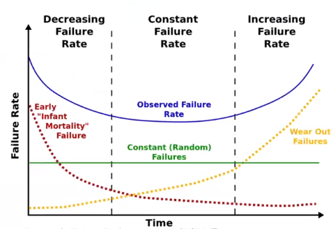
The Bathtub curve demonstrates that most failures occur either early on, or in old age as machines start wearing out.

Dependability Design Principle #

Avoid a single point of failure. A chain is only as strong as its weakest link.

Dependability behaves like Amdahl’s Law. If only a small portion of the system can be made more reliable, then the total impact is small.

Error Correction Codes (ECC) #

Memory can sometimes fail, since cells store bits and those cells are not perfect.

A soft error occurs when a bit temporarily flips (due to alpha particles etc) and can be flipped back if we recognize the error.

A hard error occurs when a cell or chip fails permanently.

In order to act upon a failure, we have to know that a failure happened in the first place. Error detection is a necessary prerequisite to redundancy.

Main idea of ECC: Add extra bits to each data-word. These extra bits are used to detect and correct faults in memory.

Hamming Codes #

The Hamming distance between two sequences of bits is the number of positions in a bitstring that differ in value from another bitstring.

One idea is to do a parity check by counting the number of “on” bits. A bitstring has an even parity if the number of on bits is even. We can use an extra bit that is flipped such that the final string always has an even parity. So, if a bitstring is checked and it has odd parity, then something is wrong! This scheme detects 1-bit errors and has a minimum Hamming distance of 2 (the error and the parity bit).

Using Hamming Codes, we can allow error correction at a minimum Hamming distance of 3. (i.e. no 2-bit error can map back to another code word.).

• Every power of 2, we add a parity bit that keeps track of the parity of the subset of bits where the index of the bit has a $1$ in a particular position.

  

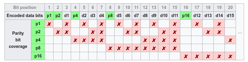
• To determine if a bitstring is correct, we check parity bits and see which ones return errors. We can then sum up the parity bit numbers to find the index of the bit that has an error. For example, if parity bits 8 and 2 return an error, then bit 10 is wrong and must be flipped.

Hash Functions #

Sometimes, we need to also protect against deliberate errors (made by hackers, etc). Cryptographic hash functions like SHA256 allow us to quickly, and with high probability, determine if two bitstrings are the same or different.

RAID #

Redundant Array of Inexpensive Disks. Rather than using one large, expensive, reliable disk, we use a large amount of small, expensive, unreliable disks and duplicate the data across the disks.

• RAID 0: No redundancy, striped volumes only. Very unreliable (any one disk failure means data loss).
• RAID 1: Disk mirroring. Every disk is fully duplicated onto its mirror. This produces a very large data availability and optimized read rates, but at the cost of needing 100% overhead.
• RAID 3: Parity disk. For every 3 disks, 1 additional disk is used to store parity information (so 1/4 of the data cost as RAID 1). If any one of the four disks fails, the data will still be intact.
• RAID 4: Disk sectors. Rather than operating at the bit level (like RAID 3), RAID 4 operates on a stripe level. Reads and writes must be done both to the original disk and the parity disk. This works well for small reads, but small writes can be problematic because every modified stripe needs to be parity checked. So the bottleneck becomes the parity disk.
• RAID 5: Interleaved parity. In a larger array, an independent set of parity disks each contain a few stripes for each drive. This cuts down on write bottlenecks since the chance of multiple drives writing to the same parity drive is reduced.
• RAID 6: RAID 5 with two parity blocks per stripe. So the drive array can tolerate 2 disk failures rather than just 1, at the cost of needing additional capacity.