Markov Decision Processes
What is a Markov Decision Process? #
A Markov Decision Process is a Markov model that solves nondeterministic search problems (where an action can result in multiple possible successor states).
A MDP is defined by:
- A set of states $s$
- A set of actions $a$
- A transition model $T(s, a, s’)$ that represents the probability $P(s’ | s, a)$ - that the action $a$ taken at state $s$ will lead to a new state $s’$. (Allowed by memoryless property)
- A reward function $R(s, a, s’)$ per transition
- Discount factor $\gamma \in [0, 1]$
- A start state
- A terminal (absorbing state)
The utility function of an MDP can be calculated as follows:
$$ U([s_0, a_0, s_1, a_1, s_2, \cdots]) = R(s_0, a_0, s_1) + \gamma R(s_1, a_1, s_2) + \gamma^2 R(s_2, a_2, s_3) + \cdots $$
Intuitively, the discount factor causes an exponential decay over time, so if an agent takes too long to reach a state it is automatically terminated. This also solves the problem of infinite reward streams. (enforce a finite horizon)
- The reward is bounded by the value $\frac{R_{\max}}{1-\gamma}$.
The primary goal for an MDP is to find an optimal policy $\pi^*$ that gives us an action for every state that results in the maximum expected utility.
- The expected utility of a policy $U^{\pi}(s_0)$ is equal to the sum over all possible state sequences multiplied by the probability of them occurring.
Solving MDPs #
The Bellman Equation #
Some values:
- The utility of a state $s$ is equal to the expected utility when starting at $s$ and acting according to the optimal policy.
- The utility of a Q-state $Q^*(s,a)$ is equal to the expected utility of taken action $a$ in state $s$, then acting optimally.
The Bellman Equation is as follows:
$$ U^(s) = \max_a \sum_{s’} T(s, a, s’)\times(R(s, a,s’) + \gamma U^(s’)) = \max_a Q^*(s, a) $$
- The equation finds the optimal value of the state $s$ by multiplying the transition probability to the next state by the reward for that transition plus the discounted utility of the next state.
- The inner sum term is equivalent to the utility of the Q-state.
- The equation creates a dynamic programming problem where the subproblem $U^*(s’)$ is used to calculate the current state’s utility.
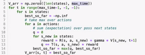
Value Iteration #
Used for computing the optimal values of states, by iterative updates until convergence.
In order to compute the value of a state. we can use the following algorithm:
- For all states $s \in S$, initialize their starting value $U_0(s) = 0$.
- Until convergence (i.e. $U_{k+1} = U_k$), run the following update formula:
- $\forall s \in S, U_{k+1}(s) = \max_a \sum_{s’} T(s, a, s’)\times (R(s, a, s’) + \gamma U_k(s’))$
- Unlike the Bellman equation, which tests for optimality, this equation changes the value iteratively using dynamic programming.
- In other words, this equation takes the max of the values of alll neighboring states, and multiplies it by the transition probability (if nondeterministic).
- $U^*(s)$ for any terminal state must be $0$ (since no actions can be taken from these states).
Properties:
- Value iteration is guaranteed to converge for discounts less than 1.
- Value iterations will converge to the same $U^*$ values regardless of initial values.
- The runtime of value iteration is $O(|S|^2 |A|)$ since for every action, we need to compute each action’s Q-value which requires iterating over all states.
Q-value iteration is a similar update algorithm that computes Q-values instead:
$$ Q_{k+1}(s,a) = \sum_{s’} T(s, a, s’) \times (R(s, a, s’) + \gamma \max_{a’} Q_k (s’, a’)) $$
- This is different because for value iteration, we select an action before transitioning, whereas in Q-value iteration, we make the transition before choosing the new state.
Policy extraction: to determine the optimal policy from optimal state values (given a state value function), we can use the following equation:
$$ \forall s \in S, \pi^(s) = \argmax_a Q^(s, a) = \argmax_a \sum_{s’} T(s, a, s’) [R(s, a, s’) + \gamma U^*(s’)]$$
Policy extraction is only optimal if the state value function is optimal. Used either after value iteration (to compute optimal policies from optimal state values) or as a subroutine in policy iteration (to compute the best policy for estimated state values).
Policy Iteration #
Policy iteration has the same optimality guarantees as value iteration, but has better performance. The algorithm is as follows:
- Define an initial policy. The closer the initial policy is to the optimal policy, the faster it will converge.
- Compute $U^{\pi}(s) = \sum_{s’} T(s, \pi(s), s’) [R(s, \pi(s), s’) + \gamma U^{\pi}(s’)]$ for all states $s$ (the expected utility of starting in state $s$ when following the current policy $\pi$).
- Generate the next iteration $i$ of policy values using the equation above for every state.
- Use policy improvement to generate a better policy: $\pi_{i+1}(s) = \argmax_a \sum_{s’} T(s, a, s’)[R(s, a, s’) + \gamma U^{\pi_i}(s’)]$
- Repeat steps 2-5 until $\pi_{i+1} = \pi_i = \pi^*$.