Chapter 8: Caching
Introduction #
At this point, we’ve solved nearly all of the problems with base and bound memory translation. But there is one major problem left— all of this additional complexity adds lots of memory accesses, which might make things very inefficient! This is where caching comes in.
Since programs only care about a very small subset of the total information available, if we identify this subset and place it into more local memory, then we can efficiently perform most memory accesses.
Caches give the benefits of speed from the fastest types of memory while still having the capacity of the largest memory. Ideally, caches are implemented such that they are invisible to programmers: they will automatically move memory between locations.
Cache Terminology #
Basic Anatomy #
Caches have tags (addresses) and blocks (aligned words that store information).
In order to simplify the comparison process (so that we don’t need to check every tag to see if we have a hit or miss), we can split the cache into sets. So we only need to compare a tag to a particular set in order to determine if we have a hit or miss.
A valid bit is flipped if a particular entry is valid. If the valid bit is not on, then we should treat an access like a cache miss.
A cache flush invalidates all entries.
The cache capacity is the total number of bytes in the cache.
A cache line, other wise known as a cache block, is a single entry in the cache.
The block size is the number of bytes in each cache line/block.
We can calculate the number of cache lines by dividing the cache capacity by the block size.
Eviction is the process of removing an entry from the cache.
Locality #
The primary purpose of caches is to benefit from locality of information, which allows data to be accessed faster in common patterns.
There are two different types of locality:
- Temporal Locality: locality in time. If a memory location is referenced, then chances are it might be needed again soon and so we should keep it around.
- Spatial Locality: locality in space. If a memory location is referenced, then chances are the addresses close to that will be needed soon and should be saved to faster memory.
Hits and Misses #
A cache hit occurs when the memory address we’re looking for is actually stored in the cahce.
A cache miss is when we are looking for information that is in the main memory, but not the cache.
- Compulsory Miss: cold start; the first time we access a block. These get to be pretty insignificant the more memory you have and the longer you run the program.
- Capacity miss: The cache cannot contain all of the blocks accessed by the program. These can be avoided by increasing the size of the cache.
- sizeof(array) > cache size
- Conflict miss (collision): Multiple memory locations map to the same cache set. These could be avoided by increasing the associativity of the cache (these would never happen with a fully associative cache).
- Related to spatial locality breakdown: when stride * sizeof(element) ≥ block size. i.e. A block is loaded, but only the first element in the block is accessed before it is overwritten by another block.
- Coherence miss: External processors or devices update a part of memory, making the cached version invalid.
Types of Caches: Associativity #
The associativity of a cache is the number of places each block is allowed to be in. Having a higher associativity increases the total cache capacity (thus reducing AMAT), but becomes more complex.
- Fully associative cache: Blocks can go anywhere. This is the most flexible option, but requires a large number of comparators (1 per block).
- Direct mapped cache: Each block goes into one place, such that each set contains exactly one block. This makes it straightforward to check if a block exists (since there is only one place it can possibly go), but is the least flexible.
- N-way Set Associative: There are N places for a block, such that each set has N number of blocks. This is a compromise between fully associative (N = # blocks) and direct mapped (N = 1).
Tags, Index, Offset: The Address #
Addresses in the cache are divided into tag, index, and offset.
Offset #
Tells us where data exists in the cache line.
Containes $\log_2(blocksize)$ number of bytes (not bits) (for example, 64 byte blocks can be represented using 6 offset bits).
Index #
Tells us the where in the cache an address might be stored.
Contains $\log_2$(num cache lines / associativity) number of bits.
For example, a 4 way associative cache with 512 lines requires 7 index bits.
Tag #
Determines which memory location in the cache that the data is stored.
The number of bits in the tag is just the bits remaining (total address bits - index bits - offset bits).
Total Cache Capacity #
Total cache capacity = Associativity $\times$ Number of Sets $\times$ Block Size
Bytes of memory in cache = blocks per set $\times$ number of sets $\times$ bytes per block
Increasing associativity: Increases hit time, decreases miss rate (less conflict misses), does not change miss penalty
Increasing number of entries: increases hit time (reading from larger memory), decreases miss rate (2x drop for every 4x increase in capacity), does not change miss penalty.
Increasing block size: does not change hit time, decreases miss rate due to spatial locality but increases conflict misses in the long run, larger miss penalty
Reducing miss penalty: Use more cache levels!
Cache Performance #
Hit Time: the amount of time needed to return data in a cache. This is usually measured in terms of cycles.
Miss penalty: The additional time to return an element if it is not in the cache.
Miss rate: The proportion of a program’s memory requests that cause a cache miss.
The main measurement of cache performance is AMAT (Average Memory Access Time).
AMAT = Hit Time + Miss Rate * Miss Penalty
For example, if a memory access takes 50ns, the cache lookup time is 5ns, and the hit rate is 90%, the AMAT would be:
$0.9 * 5 + 0.1 (5 + 50)$ which is 10ns.
We can improve AMAT by:
- Reducing the time to hit in the cache (make it smaller)
- Reduce the miss rate (bigger cache or better programs)
- Reduce the miss penalty (have multiple cache levels)
Write-through vs. Write-back #
When store instructions write to memory, we change the values. We need to then change both the cache value and the memory value to make sure that everything remains consistent.
We can use the write-through policy which states that we need to write values to both cache and memory. Since writing to memory is slow, we can instead write to a write buffer which stores the desired value until it is done being written.
The write-back policy states that we should write only to cache and then write the cache block back to memory when the block is evicted from the cache. That way, there is only a single write to memory per block, and writes are collected in the cache.
- Using the write-back policy, we include a “dirty” bit to indicate if a block was written to or not.
Write through is good because:
- It has simpler control logic.
- There is more predictable timng.
- It’s easier to make reliable since there is memory redundancy (both cache and DRAM have new values).
On the other hand, write-back:
- Is more complex, with variable timing.
- Reduces write traffic since we do fewer writes.
- Sometimes, only cache has data and so cache failure would result in disaster.
Translation Lookaside Buffer (TLB) #
To improve the performance of our address translation scheme from the previous chapter, let’s see how we can apply the concept of caches to storing recently used addresses.
We can store mappings from virtual to physical addresses in a custom cache known as the translation lookaside buffer. That way, even if we have a multi-level address translation scheme, stored addresses can be quickly accessed with no further memory lookups required.
Thrashing #
While great for reducing access times for cache hits, miss times with the TLB are very high because it exists in the critical path, and we would need additional accesses to go around it.
If the TLB is not big enough, or we otherwise keep evicting entries that are still needed, thrashing occurs, where there are continuous conflicts between accesses. To circumvent this, most TLBs are fully associative and have 128 to 512 entries.
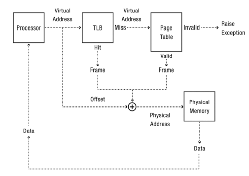
Memory Access Walkthrough #
When some data needs to be accessed from the disk, the following happens:
- Check the TLB. If the cached translation exists, then we can simply access the physical memory directly.
- Check the page table. If the page exists, then access it directly.
- Otherwise, the entry is invalid or missing and a page fault occurs.
- Load the page into memory.
- Update the page table.
- Update the TLB to point to the new page entry.
Demand Paging #
The final application of caching we’ll explore in this chapter is demand paging. In addition to storing address translations in a cache, we can also store the data from the disk itself!
The reason why this is useful is because modern computers typically do not use all of their physical memory. Thus, we can take advantage of the unused portions to speed up otherwise slow disk accesses. In other words, we use physical memory as a cache for the disk.
Demand Paging Mechanisms #
Here’s how demand paging is typically set up, in cache terms:
- The block size is typically 4KB (1 page each).
- The cache is fully associative, since it can arbitrarily map any virtual address to any physical address.
- The cache is write-back, since write-through would defeat the entire purpose of demand paging. This means we need a dirty bit in the cache.
- On a page fault, the following occurs:
- Choose an old page to replace (by a demand paging policy in the next section).
- If the old page was modified (i.e. dirty bit set), then write the contents back to the disk before evicting.
- Change the old page’s page table entry and TLB to be invalid.
- Load the new page into memory.
- Update the page table entry and invalidate the previous TLB entry for that page.
- Continue the current thread. When the thread starts, it will update the TLB.
The Working Set Model #
Every program has to access a certain amount of memory in its execution. We can call the entire set that needs to be accessed the working set. A larger proportion of cache hits generally means that a larger part of the working set is available in the cache.
- The minimum number of entries needed to store the entire working set in the TLB is (working set size)/(page size). For example, if the working set size is 256KB and the page size is 4KB, then 64 entries are required.
At any point in time, a portion of the demand paging cache (i.e. main memory) is used to store a process. We can call this the resident set size.
- If the physical memory size is less than the resident set size, then thrashing is likely to occur.