 ben's notes
Asymptotic Analysis Basics
Content Note
This concept is a big reason why a strong math background is helpful for computer science, even when it’s not obvious that there are connections! Make sure you’re comfortable with Calculus concepts up to power series.
An Abstract Introduction to Asymptotic Analysis #
The term asymptotics, or asymptotic analysis, refers to the idea of analyzing functions when their inputs get really big. This is like the asymptotes you might remember learning in math classes, where functions approach a value when they get very large inputs.
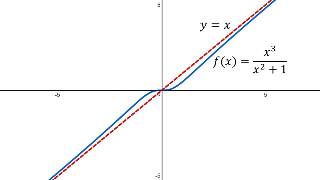
Here, we can see that $y= \dfrac{x^3}{x^2 + 1}$ looks basically identical to $y = x$ when x gets really big. Asymptotics is all about reducing functions to their eventual behaviors exactly like this!
That’s cool, but how is it useful? #
Graphs and functions are great and all, but at this point it’s still a mystery as to how we can use these concepts for more practical uses. Now, we’ll see how we can represent programs as mathematical functions so that we can do cool things like:
- Figure out how much time or space a program will use
- Objectively tell how one program is better than another program
- Choose the optimal data structures for a specific purpose
As you can see, this concept is absolutely fundamental to ensuring that you write efficient algorithms and choose the correct data structures. With the power of asymptotics, you can figure out if a program will take 100 seconds or 100 years to run without actually running it!
How to Measure Programs #
In order to convert your public static void Main(String[] args) or whatever into y = log(x), we need to figure out what x and y even represent!
TLDR: It depends, but the three most common measurements are time, space, and complexity.
Time is almost always useful to minimize because it could mean the difference between a program being able to run on a smartphone and needing a supercomputer. Time usually increases with the number of operations being run. Loops and recursion will increase this metric substantially. On Linux, the time command can be used for measuring this.
Space is also often nice to reduce, but has become a smaller concern now that we can get terabytes (or even petabytes) of storage pretty easily! Usually, the things that take up lots of space are big lists and a very large number of individual objects. Reducing the size of lists to hold only what you need will be very helpful for this metric!
There is another common metric, which is known as complexity or computational cost. This is a less concrete concept compared to time or space, and cannot be measured easily; however, it is highly generalized and usually easier to think about. For complexity, we can simply assign basic operations (like println, adding, absolute value) a complexity of 1 and add up how many basic operation calls there are in a program.
Simplifying Functions #
Since we only care about the general shape of the function, we can keep things as simple as possible! Here are the main rules:
- Only keep the fastest growing term. For example, $log(n) + n$ can be simplified to just $n$since $n$ grows faster out of the two terms.
- Remove all constants. For example, $5log(3n)$ can just be simplified to $log(n)$since constants don’t change the overall shape of a function.
- Remove all other variables. If a function is really $log(n + m)$ but we only care about n, then we can simply it into $log(n)$.
There are two cases where we can’t remove other variables and constants though, and they are:
- A polynomial term $n^c$(because $n^2$grows slower than $n^3$, for example), and
- An exponential term $c^n$(because $2^n$grows slower than $3^n$, for example).
The Big Bounds #
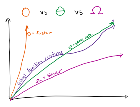
There are three important types of runtime bounds that can be used to describe functions. These bounds put restrictions on how slow or fast we can expect that function to grow!
Big O is an upper bound for a function growth rate. That means that the function grows slower or the same rate as the Big O function. For example, a valid Big O bound for $log(n) + n$ is $O(n^2)$ since $n^2$ grows at a faster rate.
Big Omega is a lower bound for a function growth rate. That means that the function grows faster or the same rate as the Big Omega function. For example, a valid Big Omega bound for $log(n) + n$ is $\Omega(1)$ since $1$ (a constant) grows at a slower rate.
Big Theta is a middle ground that describes the function that grows at the same rate as the actual function. Big Theta only exists if there is a valid Big O that is equal to a valid Big Omega. For example, a valid Big Theta bound for $log(n) + n$ is $\Theta(n)$ since $n$ grows at the same rate (log n is much slower so it adds an insignificant amount).
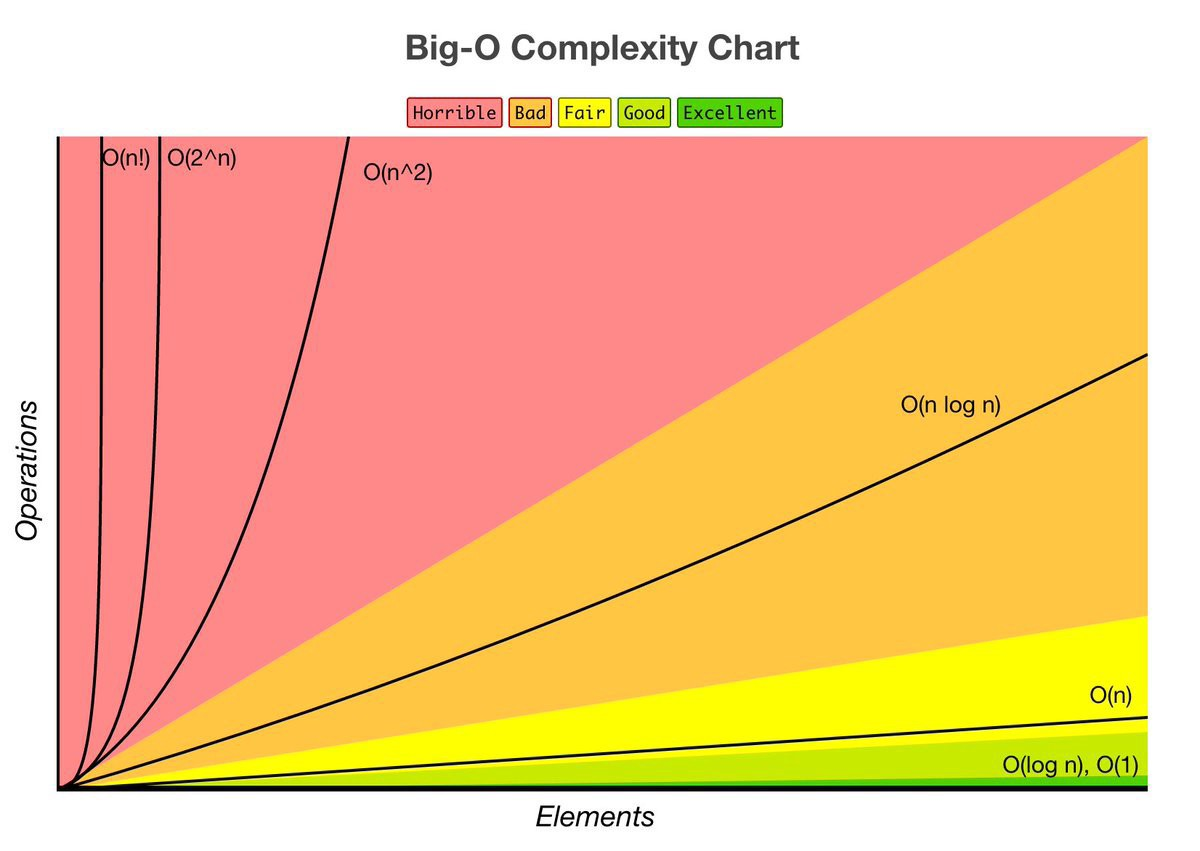
Orders of Growth #
There are some common functions that many runtimes will simply into. Here they are, from fastest to slowest:
| Function | Name | Examples |
|---|---|---|
| $\Theta(1)$ | Constant | System.out.println, +, array accessing |
| $\Theta(\log(n))$ | Log | Binary search |
| $\Theta(n)$ | Linear | Iterating through each element of a list |
| $\Theta(n\log(n))$ | nlogn 😅 | Quicksort, merge sort |
| $\Theta(n^2)$ | Quadratic | Bubble sort, nested for loops |
| $\Theta(2^n)$ | Exponential | Finding all possible subsets of a list, tree recursion |
| $\Theta(n!)$ | Factorial | Bogo sort, getting all permutations of a list |
| $\Theta(n^n)$ | n^n 😅😅 | Tetration |
Don’t worry about the examples you aren’t familiar with- I will go into much more detail on their respective pages.
Asymptotic Analysis: Step by Step #
- Identify the function that needs to be analyzed.
- Identify the parameter to use as $n$.
- Identify the measurement that needs to be taken. (Time, space, etc.)
- Generate a function that represents the complexity. If you need help with this step, try some problems!
- Simplify the function (remove constants, smaller terms, and other variables).
- Select the correct bounds (O, Omega, Theta) for particular cases (best, worst, overall).