Iterators and Joins

Introduction #

As you may have seen already, some SQL queries involve joining lots of tables together to get the data we need. However, that joining comes at a cost- every join multiplies the number of rows in the output by the number of rows in the table!

For this reason, it’s very important that we try to optimize the join operation as much as possible, such that we can minimize the amount of data to process. In this section, we’ll explore a methods of doing this, and compare their runtimes.

Tip

I would recommend playing around with the Loop Join Animations visualizer I made- it will help provide some intuition for the first few joins since staring at an algorithm isn’t for everyone!

The discussion slides also have a full walkthrough of the more involved joins (SMJ, GHJ).

Relevant Materials #

• Loop Join Animations
• Discussion 6
• Note 8

Cost Notation #

Make sure you keep this section around (whether it’s in your head, or bookmarked)! It’ll be extremely useful for this section.

Suppose $R$ is a table.

• $[R]$ is the number of pages needed to store $R$.
• $p_R$ is the number of records per page of $R$.
• $|R|$ is the number of records in $R$, also known as the cardinality of $R$.
  • $|R| = p_R \times [R]$.

Simple Nested Loop Join #

Intuitively, joining two tables is essentially a double for loop over the records in each table:

for record r in R:
	for record s in S:
		if join_condition(r, s):
			add <r, s> to result buffer

where join_condition is an optional function, also known as $\theta$, that returns a boolean (true if record should be added to result).

The cost of a simple join is the cost of scanning $R$ once, added to the cost of scanning $S$ once per tuple in $R$: $$[R] + |R|[S]$$

Page Nested Loop Join #

Simple join is inefficient because it requires an I/O for every individual record for both tables.

We can improve this by operating on the page level rather than the record level: before moving onto the next page, process all of the joins for the records on the current page.

for rpage in R:
	for spage in S:
			for rtuple in rpage:
					for stuple in spage:
						if join_condition(rtuple, stuple):
							add <r, s> to result buffer

Now, the cost becomes the cost of scanning $R$ once, then scanning $S$ once per page of $R$: $$[R] + ([R] \times [S])$$

Block Nested Loop Join #

To improve upon loop join even further, let’s take advantage of the fact that we can have $B$ pages in our buffer.

Rather than having to load in one page at a time, we can instead load in:

• $1$ page of $S$
• $1$ output buffer
• $B-2$ pages of $R$

and then load in each page of $S$ one by one to join to all $B-2$ pages of $R$ before loading in a new set of $B-2$ pages.

for rblock of B-2 pages in R:
	for spage in S:
		for rtuple in rblock:
			for stuple in sblock:
				add <rtuple, stuple> to result buffer

The cost now becomes the cost of scanning $R$ once, plus scanning $S$ once per number of blocks: $$[R] + \lceil [R] / (B-2) \rceil \times [S]$$

Index Nested Loop Join #

In previous version of nested loop join, we’d need to loop through all of the elements in order to join them.

However, with the power of B+ trees, we can quickly look up tuples that are equivalent in the two tables when computing an equijoin.

for rtuple in R:
	add <rtuple, S_index.find(joinval)>

Cost: $[R] + |R| \times t_S$ where $t_S$ is the cost of finding all matching $S$ tuples

• Alternative 1 B+Tree: cost to traverse root to leave and read all leaves with matching utples
• Alternative 2/3 B+Tree: cost of retrieving RIDs + cost to fetch actual records
  • If clustered, 1 IO per page. If not clustered, 1 IO per tuple.
• If no index, then $t_S = |S|$ which devolves INLJ into SNLJ.

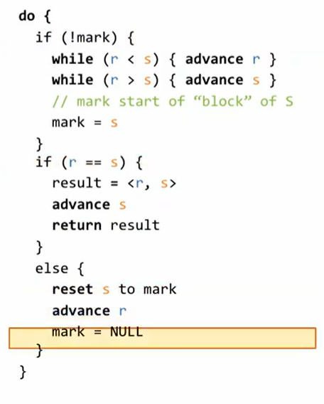
Sort-Merge Join #

Main idea: When joining on a comparison (like equality or $<$), sort on the desired indices first, then for every range (group of values with identical indices) check for matches and yield all matches.

The cost of sort-merge join is the sum of:

• The cost of sorting $R$
• The cost of sorting $S$
• The cost of iterating through R once, $[R]$
• The cost of iterating through S once, $[S]$

One optimization we can make is to stream both relations directly into the merge part when in the last pass of sorting! This will reduce the I/O cost by removing the need to write and re-read $[R] + [S]$. This subtracts $2 \times ([R] + [S])$ I/Os from the final cost.

Grace Hash Join #

If we have an equality predicate, we can use the power of hashing to match identical indices quickly.

Naively, if we load all records in table $R$ into a hash table, we can scan $S$ once and probe the hash table for matches- but this requires $R$ to be less than $(B-2) \times H$ where $H$ is the hash fill factor.

If the memory requirement of $R < (B-2) * H$ is not satisfied, we will have to partition out $R$ and process each group separately.

Essentially, Grace Hash Join is very similar to the divide-and-conquer approach for hashing in the first place:

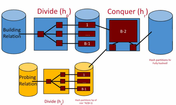
• In the dividing phase, matching tuples between $R$ and $S$ get put into the same partition.
• In the conquering phase, build a separate small hash table for each partition in memory, and if it matches, stream the partition into the output buffer.

Full process:

1. Partitioning step:
   1. make $B-1$ partitions.
   2. If any partitions are larger than $B-2$ pages, then recursively partition until they reach the desired size.
2. Build and probe:
   1. Build an in-memory hash table of one table $R$, and stream in tuples of $S$.
   2. For all matching tuples of $R$ and $S$, stream them to the output buffer.

Calculating the I/O Cost of GHJ #

The process of calculating the GHJ cost is extremely similar to that of standard external hashing. The main difference is that we are now loading in two tables at the same time.

Let’s look at the example from Discussion 6:

• Table $R$ has 100 pages and 20 tuples per page.
• Table $S$ has 50 pages and 50 tuples per page.
• Assume all hash functions partition uniformly.
• Do not include the final writes in the calculation.
• If $B=8$, what is the I/O cost for Grace Hash Join?

Number of Passes #

Like hashing, our goal is to make the partitions small enough to fit in the buffer. But now that we have two tables, we only need one of them to fit! This is because we can put the smaller table into memory, then stream the larger table in one page at a time using one buffer frame.

As you can see in the image above, as long as one of the tables fits in $B-2$ pages, we’re all set for the Build and Probe stage.

In each stage, of the Partitioning step, we create $B-1$ partitions, so we solve for the number of recursive passes $x$ in the following manner: $$\lceil \frac{\min([R], [S])}{(B-1)^x} \rceil \le B-2$$ In this case, $[S]$ is smaller, so we can plug in $\lceil 50/(8^2) \rceil = 1 \le 8$ to confirm that we need $2$ passes of partitioning before we can Build and Probe.

Partition Cost #

The partition cost calculation is the same as for hashing. However, we must partition both tables separately using $B-1$ partitions each at each step.

Pass 1:

1. The first read takes $100+50 = 150$ I/Os.
2. Partition $R$ into $7$ equal partitions of $15$ and write it back to disk = $15*7=105$ I/Os.
3. Partition $S$ into $7$ equal partitions of $8$ and write it = $8*7=56$ I/Os.

Pass 2:

1. We read in the results from pass 1: $105 + 56 = 161$ I/Os.
2. Partition each of the 7 partitions of 15 into 7 more partitions of $\lceil 15/7 \rceil = 3$, making $49$ partitions of size $3$ in total. Writing these back takes $49*3 = 147$ I/Os.
3. Do the same thing for the 7 partitions of 8 to get $49$ partitions of size $2$, taking $49*2 = 98$ I/Os to write back.

Build and Probe: Building and probing requires reading all of the partitions created in pass 2. This takes $(349) + (249) = 245$ I/Os. Remember that we don’t count the final writes!

Total: $(150 + 105 + 56) + (161 + 147 + 98) + 245 = 962$ I/Os to run GHJ.