Query Optimization
Introduction #
Query optimization is the bridge between a declarative language (like SQL, where you describe “what” you want) and an imperative language (like Java, which describes how the answer is actually computed). Here, we built the translator that converts SQL into logic that a computer can understand.
If you think about it, this can be really complicated- there’s lots of ways to execute a query (i.e. many equivalent relational algebra statements), and we have to somehow figure out which one is the best without executing any of them!
Relevant Materials #
System R Optimizers #
The System R query optimizer framework was conceptualized in the 1970s, and lays the framework for most modern query optimizers today. This is what we will be studying in this class.
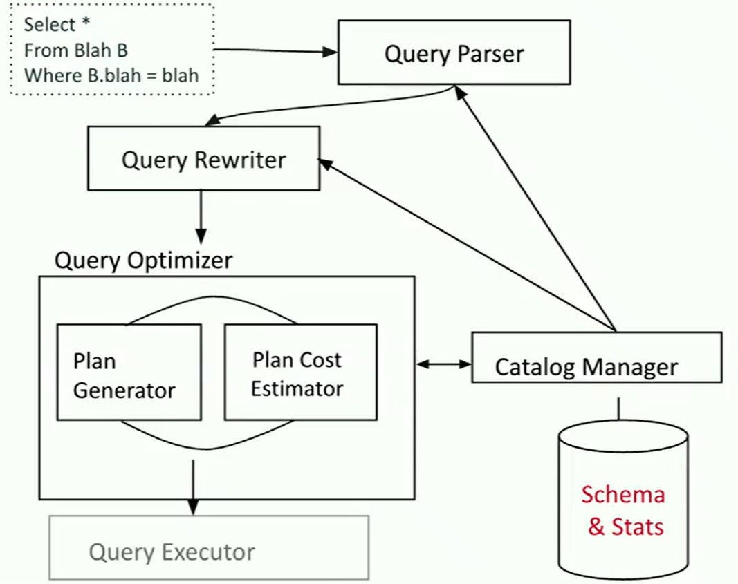
In System R, the query parser first checks for correctness and authorization (user permissions to access the table). It then generates a parse tree out of the query. This step is usually fairly straightforward, since it’s just breaking up the query into chunks that our programming language can understand, without having to make any decisions.
Next, the query rewriter converts queries into even smaller query blocks (like a single WHERE clause), and flattens the views.
Once the query is rewritten, it gets passed into the query optimizer. The primary goal of a query optimizer is to translate a simple query plan into a better query plan. A cost-based query optimizer processes one query block at a time (e.g. select, project, join, group by, order by).
For each block, consider:
- all relevant access methods
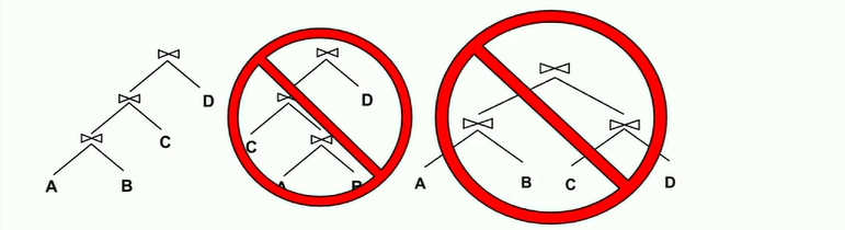
- All left-deep join trees: right branches are always simple FROM clauses. Observe the illustration below for examples of left-deep and not-left-deep trees:
Typically, we don’t care about exact performance; the main purpose of query optimization is to prune out extremely inefficient options. As long as the final result is good enough, we’re happy!
The Components of a Query Optimizer #
There are three main problems:
- Plan space: for a given query, what plans are considered?
- Two query plans are physically equivalent if they result in the same content and the same physical properties (primarily sort order and hash grouping).
- Cost estimation: how do we estimate how much a plan will cost?
- In System R, cost is represented as a single number:
I/Os + CPU-factor*#tuples(where CPU factor is the proportion of time the system spends actually computing the query). For the purposes of this class, we’ll only focus on the I/O cost. - For each term, determine its selectivity (size of output / size of input). Lower selectivity value is better (filters more items).
- Result cardinality is equal to the max number of tuples multiplied by the product of all selectivities.
- If searching for
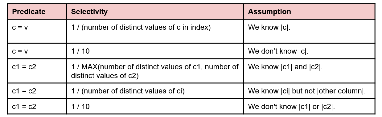
col = value, where is the number of unique values in the table. - If searching for
col1 = col2, then . - If searching for
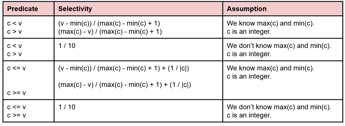
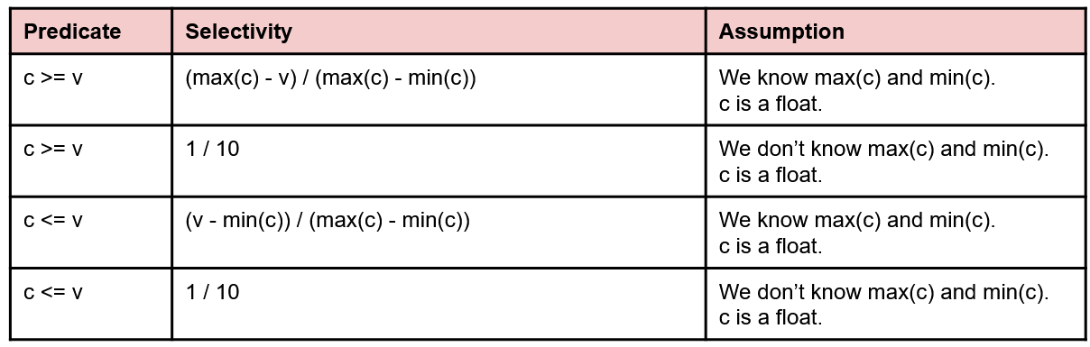
col > value, then - If we are missing the needed stats to compute any of the above, assume that .
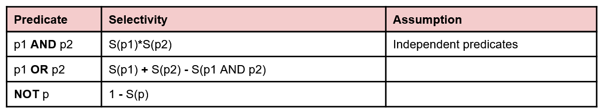
- If searching for a disjunction (or) , .
- If searching for a conjunction (and) , .
- If searching for a negation (not), , .
- For joins, simply apply the selectivity query to the cross product of the two tables that are being joined.
- For clustered indexes, the approximate number of IOs is where is the number of pages and is selectivity.
- For unclustered indexes, the approximate cost is where is the number of tuples.
- A sequential scan of a file takes cost.
- In System R, cost is represented as a single number:
- Search strategy: how do we search the plan space?
Selectivity Estimation #
Since the number of rows in our output depends heavily on the data and what selections we make out of it, we need a way to estimate the size of outputs after each operation. This is known as selectivity estimation.
Like evaluating query cost, selectivity estimation is very rough and generally prioritizes speed over accuracy- so much so that if we don’t have enough information, we just assign an operation the arbitrary selectivity value of (meaning that the the output has 1/10 of the number of rows as the input).
Below are some charts from discussion of some common cases you might run into, and how to calculate their selectivity. Assume the following:
|c|corresponds to the number of distinct values in column c.- If we have an index on the column, we should also know
|c|, and the max/min values.
To get the number of records in the output, we take the floor of the result of multiplying the selectivity estimate with the number of records in the input.
Selectivity Estimation Practice #
Suppose has 1000 tuples and has 500 tuples. We have the following indexes:
- R.a: 50 unique integers uniformly distributed in
- R.b: 100 unique float values uniformly distributed in
- S.a: 25 unique integers uniformly distributed in
What is the estimated number of tuples in the output after running the following queries?
SELECT * FROM R;SELECT * FROM R WHERE a = 42;SELECT * FROM R WHERE c = 42;SELECT * FROM R WHERE a <= 25;a are less than 25 (exact formula listed above). So tuples.SELECT * FROM R WHERE b <= 25;Common Heuristics #
Selection and projection cascade and pushdown: apply selections () and projections () as soon as you have the relevant tables. i.e. push them as far to the right as possible
Avoid Cartesian products: given a choice, do theta-joins rather than cross products.
Put the more effective selection onto the outer loop before a join: reorder joins such that we are joining a smaller table in the outer loop with a larger table in the inner loop, especially if this allows us to filter out more rows in the outer loop
Materialize inner tables before joins: rather than calculating selections on the fly, create a temporary filtered table before passing it into a join
- Not effective 100% of the time since it costs IO’s to write and re-read the table
Use left-deep trees only (explained in an earlier section).
Selinger Query Optimization #
The Selinger query optimization algorithm uses dynamic programming over passes (where is the number of relations).
In each of the passes, we use the fact that left-deep plans can differ in the order of relations, access method for leaf operators, and join methods for join operators to enumerate all of the plans.
More specifically:
- In the 1st pass, find the best single relation plan for each relation. (what’s the best way to scan a table?)
- This includes full scans (# IOs = # pages in table) and index scans (# IOs depends on type of index and any applicable selects, since selections are pushed down)
- In each ith pass, find the best way to join the result of an relation plan to the th relation. (The plan will always be the outer relation due to the left-deep property.)
- For each subset of relations, retain only:
- Cheapest plan overall for each combination of tables,
- Cheapest plan for each interesting order of tuples
The principle of optimality: the best overall plan is composed of the best decisions on the subplans. This means that if we find the cheapest way to join a subset of tables, we can add on more tables one by one by finding the cheapest cost for that single join operation.
Choosing Join Algorithms #
Table access with selections and projections:
- Heap scan
- Index scan if available
Equijoins:
- Block nested loop join when simple algorithm needed
- Index nested loop join if one relation is small and the other one is indexed
- Sort-merge join if equal-size tables, small memory
- Grace hash join if 1 table is small
Non equijoins:
- Block nested loop join
Interesting Orders #
If a GROUP BY or ORDER BY clause will be processed later on, or a future join might benefit from the structure of the current join, it may be useful to take a temporary hit in IO cost in order to avoid needing to resort or regroup the table in a future step.
Only Sort Merge Join, Grace Hash Join, and index scans can produce interesting orders.
Full Sellinger Walkthrough #
This problem is taken from Fall 2020 Midterm 2.
Suppose we have the following query:
SELECT R.a, S.b, T.c
FROM R INNER JOIN S ON R.a = S.a
INNER JOIN T ON R.b = T.b
WHERE R.b <= 10 AND T.c <= 20
GROUP BY S.b;
Pass 1 #
We’re given the following possible single table access plans for Pass 1:
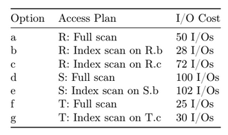
(In reality, we’d need to do selectivity estimation to find those numbers, but since you already did some practice) we’ll skip it for now.)
The first step is to identify the minimum cost accesses for each of the tables:
- Option (b) is the best way to access , so we’ll keep it.
- Option (d) is the best way to access , so we’ll keep it.
- Option (f) is the best way to access , so we’ll keep it.
Next, we can identify any interesting orders:
- The only interesting order is (e), since we
GROUP BY s.b, and (e) is an index scan on the same column.
In summary, four plans would advance: b, d, e, f.
Pass i #
Now for the 2nd pass, we will consider some ways to join two tables together:
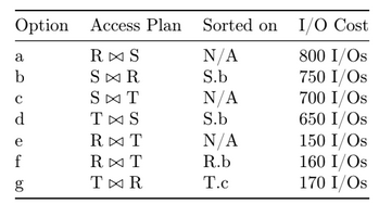
Let’s start again by identifying the best way to join each combination of tables together:
- (b) is the best way to join with .
- (d) is the best way to join with .
- (e) is the best way to join with .
However, we can see that the original query does not actually join S with T! So we can safely discard (d), since we’ll never end up using it.
Since there are no interesting orders here besides (b), the final result is that only (b) and (e) advance to Pass 3.