Causality

Prediction vs Causality #

Prediction: using $X$ data, can we guess what $y$ will be?

Causation: does X cause y to change?

• Affects decisions
• Typically established via randomized experiments

Case Studies in Causality #

Confounding Factor #

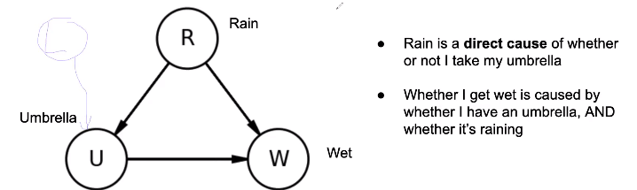
A Martian comes to Earth and observes that people using umbrellas have a higher probability of getting wet than people who do not. They infer that using an umbrella causes people to get wet.

This is an example of a confounding factor (rain) impacting both the independent and dependent variables. In reality, this third factor explains both of the observed factors (umbrella usage and getting wet)

Time and Causality #

Another martian observes that movies at a movie theater start after a group of people arrive and sit down. They conclude that people sitting down causes the movie to start.

This is an example of causality not always going forward in time: in this case, the movie being scheduled for a certain time actually caused the people to arrive and sit down, not the other way around.

Zero correlation #

A third martian observes an expert sailor moving the rudder a lot, as the boat continues in a straight line despite heavy winds. The martian concludes that moving the rudder has no effect on the direction of the boat.

This is an example of variables with zero correlation still having a causal relationship.

Structural Causal Models #

Structural Causal Models (SCMs, Graphical Models, Causal DAGs) are similar to 04 Bayes Nets, except that arrows show causality in addition to dependence.

Quantifying Association #

Pearson Correlation Coefficient #

The Pearson Correlation Coefficient $\rho_{Z,Y}$ between two variables $Z$ and $Y$ can be described below: $$\rho_{Z,Y} = \frac{cov(Z,Y)}{\sqrt{var(Z)var(Y)}}$$ where $cov(X,Y)$ is the covariance. $\rho$ is between -1 (perfect negative correlation) and 1 (perfect correlation).

Regression Coefficient #

Suppose we have a linear regression $Y = \alpha + \beta Z + \epsilon$. $\epsilon$ is the error, where $E[\epsilon] = 0$ and $cov(Z, \epsilon) = 0$.

The regression coefficient $\beta$ is described as follows: $$\beta = \rho_{Z,Y} \cdot \frac{\sigma_Y}{\sigma_Z} = \frac{cov(Z,Y)}{var(Z)}$$

If we introduce another variable (i.e. $Y = \alpha + \beta Z + \gamma X)$, then $\beta$ describes the effect of $Z$ on $Y$ while adjusting for the effects of $X$.

Risk Differences and Risk Ratio #

If in a binary situation (either the result $Y$ is $1$ or $0$), then we can quantify association using three methods:

Risk Difference: $P(Y=1|Z=1) - P(Y=1|Z=0)$ Risk Ratio: $P(Y=1|Z=1)/P(Y=1|Z=0)$ Odds Ratio: $$\frac{P(Y=1|Z=1)/P(Y=0|Z=1)}{P(Y=1|Z=0)/P(Y=0|Z=0)}$$

Paradoxes #

Simpson’s Paradox #

Aggregated data and disaggregated data create different conclusions.

For example, suppose two restaurants were rated as follows: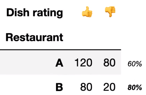 Clearly, Restaurant B is better since it received a higher ratio of positive reviews.

However, if we break up the data by year, the following is observed: 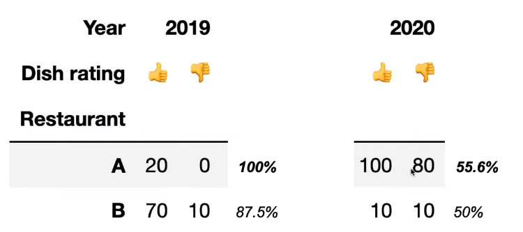Now, Restaurant A looks clearly better since it performed better in both 2019 and 2020.

Simpson’s Paradox isn’t really a paradox, since it just occurs due to a confounding variable. In the example above, the confounding variable is the effect of the COVID-19 pandemic on making reviews more negative overall: 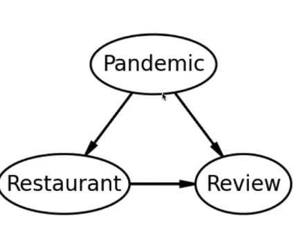If we only look at the bottom half of this causal DAG, we can observe the results that we saw above without understanding why it occurs.

If a confounding variable is present, we should condition on it and draw conclusions based on the disaggregated results.

Berkson’s Paradox #

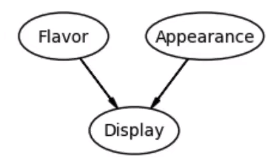
Berkson’s Paradox is very similar to Simpson’s Paradox, but acts on a collider variable rather than a confounding variable.

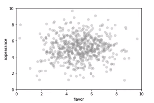
For instance, only plotting perceived flavor with perceived appearance for bread at a bakery could seem to show no correlation:

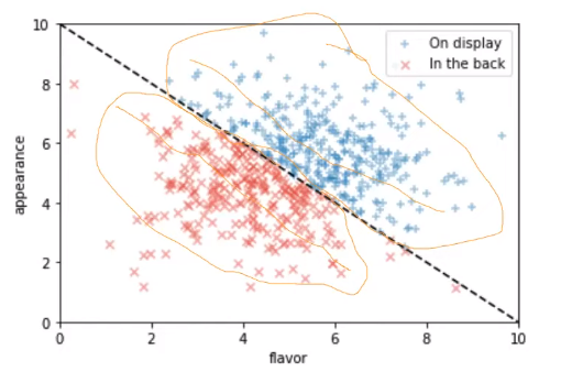
However, if we split the bread on display with the bread in the back, the following occurs:

The DAG looks like the following.

Potential Outcomes Framework #

In the Potential Outcomes Framework, we construct universes under the assumption that no confounding variables exist.

Suppose we have two universes, 0 and 1, where one has a treatment and one has a control in completely identical conditions. The outcomes are Y(0) and Y(1) respectively. The Individual Treatment Effect is equal to $Y(1) - Y(0)$.

This attempts to mitigate the fundamental problem of causal inference, which is that we can never truly compute the individual treatment effect in the real world since it’s impossible to fully replicate a particular situation and only change one variable.

Since the ITE is impossible to compute, we’ll try to find the average treatment effect (ATE), $E[Y(1) - Y(0)]$, which expands to $E[Y(1) | Z=1] P(Z=1) - E[Y(0)|Z=1] P(Z=1) + E[Y(1)|Z=0] P(Z=0) - E[Y(0)|Z=0]P(Z=0)$. In most cases, this value is also impossible to compute because of the non-matching $Y$ and $Z$ terms (in the treatment case, what would have happened if they didn’t actually receive the treatment).

An attempt to make this computable is the Simple Difference in Observed Means (SDO) which is simply $E[Y(1)|Z=1] - E[Y(0)|Z=0]$. This would only be equal to the ATE if $Y$ and $Z$ are independent (if $A$ and $B$ are independent, then $E[A|B] = E[A]$). This is true in a randomized experiment.

A unit is a single data point that we’re trying to make causal inferences on. For example, the unit in a drug test could be one person.

• Each unit has three random variables $(Z_i, Y_i(0), Y_i(1))$ where $Z$ is $1$ if the treatment was applied, $0$ otherwise.
• superpopulation model: units are i.i.d. (newer framework)
• fixed-sample model: $Z_i$ are i.i.d, $Y$ are fixed and unknown (traditional)

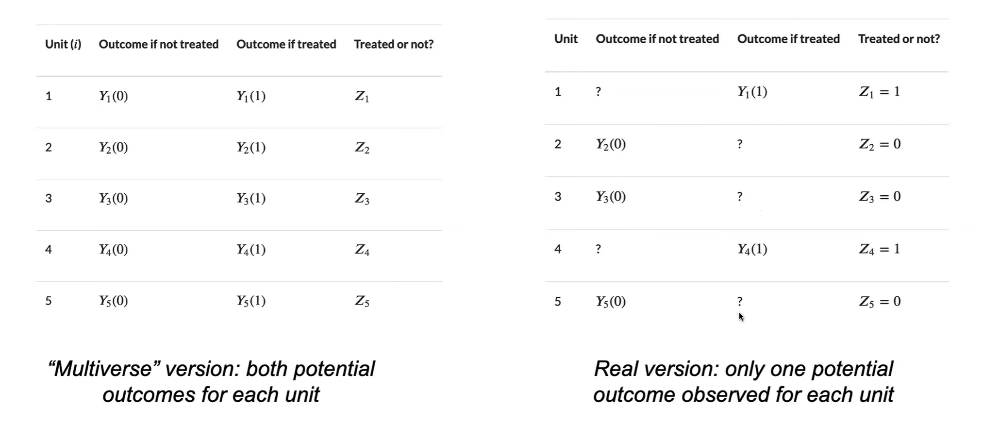
Science Table: displays units in a table. In reality, we can’t observe the $Y$ corresponding to the outcome that didn’t happen; the problem we need to solve is how we can fill these values in.

Stable Unit Treatment Value Assumption (SUTVA):

• The same treatment is applied to all units
  • Example: surgery outcomes do not follow this assumption because some surgeons could be more skiilled than others
• Units do not affect each other
  • Example: social media influencers may affect the behaviors of their followers

Causal Inference in Observational Studies #

Since we can’t truly randomize treatments in observational studies, it’s often difficult to find causality.

There are two main categories of methods for establishing causal inference:

Unconfoundedness (conditional independence): Consider all confounding variables $X$, then assume $Z$ and $Y$ are conditionally independent given $X$.

• Matching, outcome regression, propensity weighting

Natrual experiments: Find natural sources of randomness and use these to get around the confound

• Instrumental variables, regression discontinuity, difference in differences

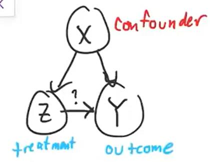
Linear Structural Model #

$$Y = \alpha + \beta X + \tau Z + \epsilon$$

• $E[\epsilon] = 0$, and $\epsilon$ is independent of $Z$ and $X$.
• $X$ is the confounder, $Y$ is the outcome, and $Z$ is the treatment.
  • 
• Assume we can’t know $X$ (too many considerations).
• The ATE is equal to $\tau$.
• Using ordinary least squares, $\hat\tau = cov(Y,Z)/var(Z) = cov(\tau Z, Z)/var(Z) + cov(\beta X, Z)/var(Z)$. $$\hat\tau_{OLS} = \tau + \beta \frac{cov(X,Z)}{var(Z)}$$ where the second term is the omitted variable bias.

Instrumental Variables #

If there exists a truly random variable $W$, we may be able to take advantage of it in the model above. Certain conditions are required:

• W is independent of $X$.
• $W$ only affects $Y$ through $Z$. One example of an instrumental variable is the Vietnam War draft lottery system, where individuals were selected for service based on their birthday. This would directly affect whether or not the individual served in the lottery independent of other confounding factors, which could then be used to establish causality between military service and another variable.

Simple ratio of regression coefficients:

• First, fit $Z$ from $W$ to get $\gamma$.
• Then, fit Y from W to get $\tau \times \gamma$.
• Divide the two values to get $\tau$ which is equal to the ATE.

Two Stage Least Squares: first predict $Z$ from $W$, then fit $Y$ from the predictions of $Z$ to get $\tau$ (ATE). $$Y = \alpha + \beta X + \tau Z + \epsilon$$ $$Z = \alpha’ + \gamma W + \eta X + \delta$$

Conditional Independence Assumption #

If we know the confounder, then the treatment and potentials might be independent (Z is independent of Y given X). This is also known as unconfoundedness.

Let the Conditional ATE be equal to $\tau(x) = E(Y(1) - Y(0) | X=x)$ such that $\tau = E(\tau(X))$ by the tower property.

Outcome regression: compute $\tau(x)$ for every $x$ and take the average. This is simple for binary variables or linear relationships (where $Y = aX + \tau Z)$, but is difficult for nonlinear or higher dimensional relationships.

Matching: for every treated unit where $Z_i = 1$, find an untreated unit that has the same confounder values, and subtract their $Y$ values to estimate individual effect. Repeat this for every untreated unit, and average overall units to estiamte ATE.

This only works if there happen to be exact matches; approximate matching gets messy and requires additional assumptions.

Inverse Propensity Score Weighting #

Main idea: reweight the population to approximate the true potential outcome averages E(Y(0)) and E(Y(1)).

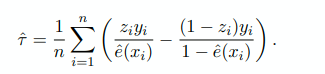IPW formula: 4 possibilities for values of $y_i$ and $z_i$. Sum up number of times each possibility occurs and divide them by how likely they are to be treated ($e(x)$).

• The propensity score $e(X) = P(Z=1|X=x)$
• Strategy:
  • make a table of all possible values of X and Z
  • divide each one by how likely it is to occur, and sum them all together
  • divide the whole result by $n$