Nonparametric Methods

What does nonparametric mean? #

Nonparametric methods make no assumptions about the distribution of the data or parameters; the null hypothesis is solely generated based on the data.

In some other contexts, the number of parameters in a nonparametric method is either infinite or grows with the number of data points.

Supposing the true state of the world is $\theta$ and our data is $x$, parametric/forward models attempt to make some assumptions about $\theta$ that make us most likely to see the data $x$. Nonparametric models go the other direction, allowing us to directly infer $\theta$ based on the observed data.

Logistic Regression vs K-Nearest Neighbors #

Logistic regression is the example of a parametric model, where we try to categorize inputs into either 0 or 1:

$$y = \sigma(\beta_1 x_1 + \beta_2 x_2 + \cdots + \beta_k x_k)$$ In this case, we must assume several things, such as linearity of data and the fact that the distribution can be roughly modelled using a sigmoid function.

Pros:

Simple (only $k$ parameters needed)
Interpretable (gives either 0 or 1 as output)
Convex loss function (guarantees an answer)
Easy to solve

Cons:

Makes assumption of linear data
Requires feature engineering to model complex/nonlinear data
Too simple for some data sets

On the other hand, K-nearest neighbors finds the $k$ points in the training set closest to a particular value, and uses majority vote at their $y$ values. KNN makes no assumptions about the underlying distribution other than that the training data is representative of the population/test data.

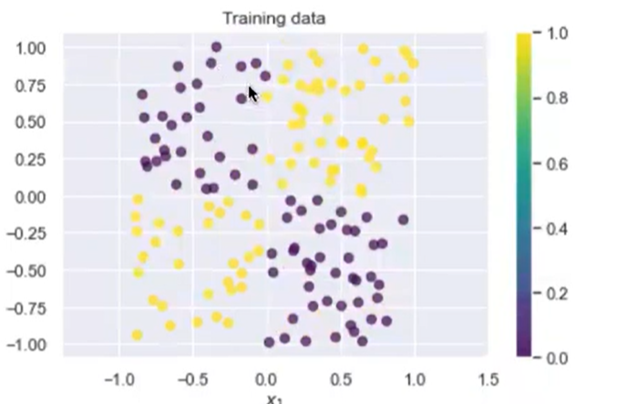
Here’s an example of some data that’s not linearly separable in which logistic regression fails, but KNN is effective:

Pros:

No assumptions made about the data/world
Simple algorithm

Cons:

Must save all training points
More difficult to interpret results (less compelling explanation)

Decision Trees #

Start at some value $(x_1, x_2, \cdots, x_n)$. Decide which feature $i$ to split on, and create two paths, for $x_i < z$ and $x_i > z$ where $z$ is some meaningful boundary. Repeat the previous step, making a binary decision once for each feature.

Decision trees are very effective if clear boundaries exist in between data of different categories, but they are sensitive to variability in the data set. To mitigate this issue, we can take multiple decision trees, and average all of their results.

Random Forests #

Using bootstrap aggregation (bagging), do the following:

independently train a large number of trees on a bootstrap sample of the data using a subset of the features.
Specifically, if there are $K$ features, each tree gets $K/3$ features if performing regression and $\sqrt K$ features for classification.

Random forests also have the benefit of controlling the depth of trees: when there are thousands of features, using a single decision tree would have an incredibly large number of decisions to make.

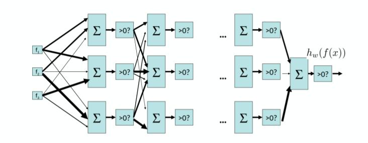
Neural Networks #

General idea: Combine multiple simple regression models together to increase complexity of the overall model.

Gradient Ascent and Descent #

The difference: gradient ascent maximizes a log-likelihood function; gradient descent minimizes a loss function.

Gradient Ascent algorithm:

randomly init w
while w not converged:
	for weight in w:
		weight = weight + learning_rate * gradient(log_likelihood(w), weight)

convergence is when gradient = 0, or no change occurs between two runs
$w$ is a vector of $N$ weights
gradient(log_liklihood(w), weight) represents the operation $\nabla_{weight} \log l(\bold{w})$, which returns a vector of $N$ partial derivatives $\partial_{weight} \log l(w_i)$ for every weight $w_i$.

Gradient Descent algorithm:

randomly init w
while w not converged:
	for weight in w:
		weight = weight - learning_rate * gradient(loss(y, x, w), weight)

Basically the same as gradient ascent, except subtract the gradient of loss instead of adding the gradient of log likelihood.

Stochastic gradient ascent/descent: only take one data point at a time to calculate the gradient. May cause inaccurate results.

Batch gradient ascent/descent: Randomly takes a batch size of $m$ data points each time to compute the gradients. Good compromise in terms of performance and accuracy.

Multilayer Perceptron #

Main idea: make perceptrons take outputs from other perceptrons as their input.

Untitled

Universal functional approximator theorem: a two-layer neural network with enough neurons can approximate any continuous function to any desired accuracy.

In order to approximate nonlinear functions, each layer is separated by a nonlinear operator. Traditional neural nets have used the sigmoid function $\sigma(x) = \frac{1}{1 + e^{-w^Tx}}$, but due to faster computation the ReLU (rectified linear unit) function is often used instead. The graphs of these two functions are as follows:

For every layer, we wrap the parameters around a function call. For example, here is a 2-layer network:

$$ f(x) = relu(x \cdot W_1 + b_1) \cdot W_2 + b_2 $$

$x$ is an $1 \times i$ input vector
$W_1$ and $W_2$ are $i \times h$ weight parameter matrices, where $h$ is the hidden layer size parameter
$b_1$ and $b_2$ are $1 \times h$ bias parameter vectors

🗒️ Ben's Notes