Regression and GLMs

Posterior Predictive Distribution #

Posterior Predictive Distribution: “if we saw some data, what future data might we expect?”

• $P(x_{n+1}|x_1,\cdots,x_n)$ = $\int P(x_{n+1}|\theta)P(\theta|x_1,\cdots,x_n)d\theta$
• $= E_{\theta|X}(P(x_{n+1}|\theta))$, which is an average with respect to the posterior.

In practice, the posterior component is estimated.

Linear Regression #

$$Y = X\beta + \epsilon$$ where $Y$ is a $n \times 1$ vector, $X$ is a $n \times d$ matrix,

• $Y$ is unknown and fixed,
• $X$ is known and fixed,
• $\epsilon$ is unknown and random (sampled from i.i.d Normal distributions).

We can calculate the squared ($L_2$) loss by using $L = \frac{1}{n}||Y-X\beta||^2$ to find that $\hat\beta = (X^TX)^{-1}X^TY$.

The distribution of Y is Normal, centered around $X\beta$ with the same variance as $\epsilon$ which is a Normal($0, \sigma^2 I_N$) distribution: $$Y \sim N(X\beta, \sigma^2I_N)$$

Nonlinear Regression #

In linear regression, we assume that the error is normally distributed. However, when the model is not linear, the error may not be normal.

Bayesian regression creates models whose parameters are described by distributions rather than exact values.

Normal distribution is more sensitive to outliers, which can increase the spread

Poisson distribution assumes that the mean and variance of the distribution are roughly the same. If the variance is actually much greater than the mean, overdispersion can occur.

Generalized Linear Models (GLMs) #

Some things that many common regression models (linear, logistic, etc) have in common:

• The data $X$ is linearly transformed by $\beta$.
• The value $X^T\beta$ is transformed using some function. (The inverse of this function is known as the link function.)
• $f(X^T\beta)$ is a parameter to some probability model.

GLMs Step by Step #

1. Formulate prediction problem: define $X$ and $Y$
2. Gather training data in (x, y) pairs
3. Choose an inverse link function and likelihood that makes sense
4. Fit model using training data (using pymc3)
5. Verify that the model is a good fit for the data (use )
6. Generate predictions when y is unknown
7. Report uncertainty for new predictions (use )

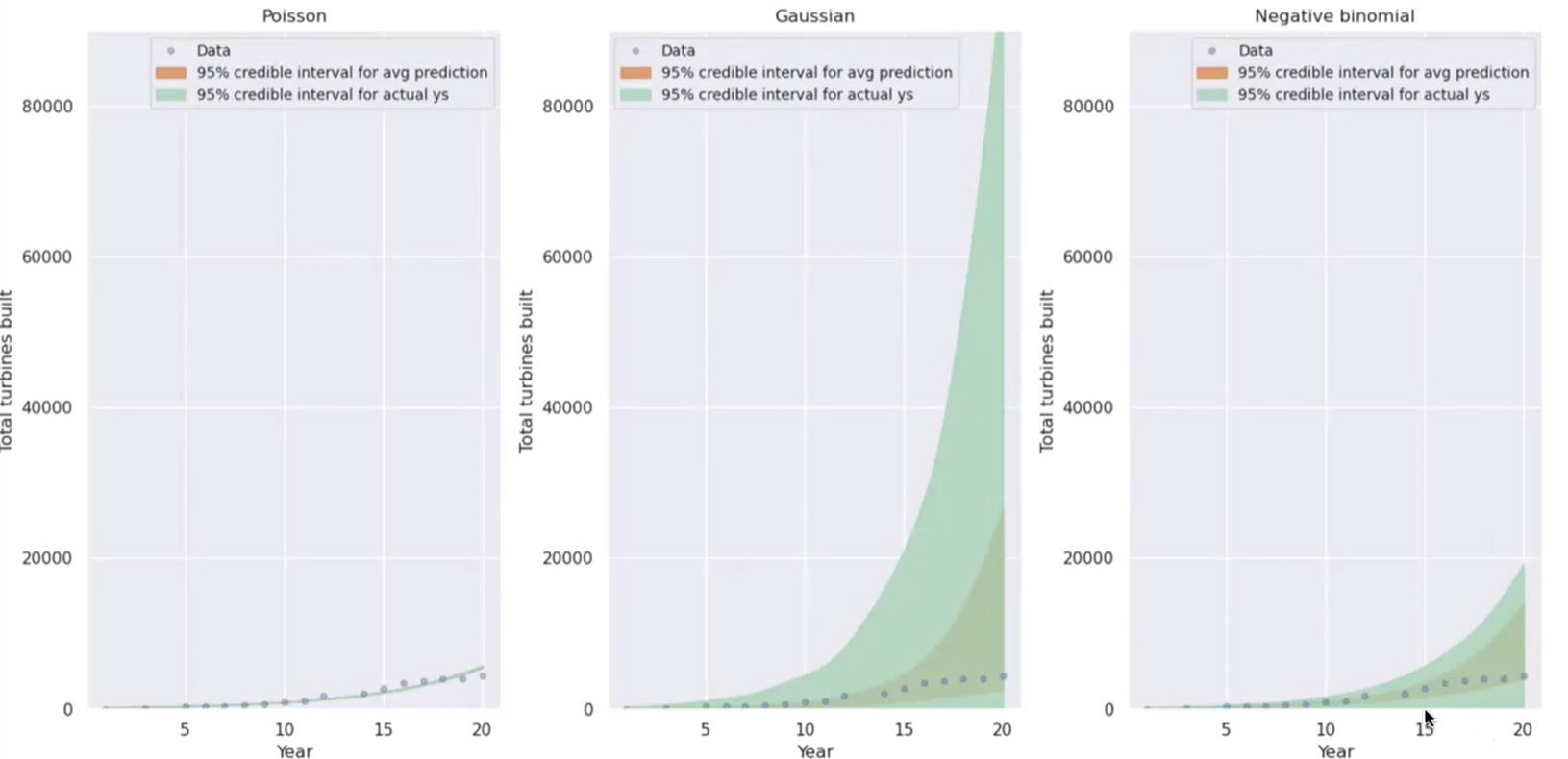
Credible Intervals #

Credible intervals are a way to quantify our uncertainty after applying a posterior distribution to test data. They are the Bayesian equivalent of confidence intervals.

A $X$% credible interval is any $X$% mass density under the posterior distribution for a parameter. It can be interpreted as “according to the posterior distribution, there is an $X$% chance that the parameter lies within this interval”.

Credible intervals are not unique, since we can choose any value to be the lower bound. However, we are primarily interested in the narrowest credible interval (since this would have the most certainty). The narrowest credible interval is known as the highest posteior density (HPD) interval, or sometimes the Highest density interval (HDI).

Ideally, we want credible intervals to be just wide enough to capture the total range of known data, while having a relatively small uncertainty. In the example below, Poisson is too narrow and Gaussian is too wide; negative binomial fits the data well.

Model Checking #

In order to determine if a model is a good fit for our data, we need to 1) make sure it fits the training data, and 2) evaluate it on new data.

Posterior Predictive Check:

1. sample from posterior
2. sample $Y’|X$ (posterior predictive distribution)
3. Check if $Y’$ looks like $Y$

Goodness of Fit for Frequentist Models #

1. Look at log-likelihood of the data
   • Problem: very hard to compare between log-likelihoods of different function classes
2. Chi-Squared Statistic: quantifies two layers of uncertainty in both the inverse link function and the likelihood model
   • In frequentist models, the parameter $\beta$ is fixed and unknown. We can estimate it using MLE: $$\hat\beta_{MLE} = argmax_\beta \\ Likelihood(y|x,\beta)$$
   • The chi-squared statistic can be calculated as such: $$\sum_i\frac{(y_i - InvLink(x_i^T\hat\beta))^2}{var(y|x_i, \beta)}$$ where the $InvLink \cdots$ term is equivalent to $E[y|x_i, \hat\beta]$.

• An ideal chi-squared value should be equal to $n$ (the number of observations made) minus the number of parameters in $\beta$. If the chi-squared is much higher than this, then the model is a poor fit for the data.

Quantifying Uncertainty in Frequentist Models #

Main idea: even though the parameter we’re estimating is fixed in frequentist settings, the estimate is random (due to it depending on the data). Therefore, we can quantify uncertainty using the distribution of the random estimate.

Central Limit Theorem: http://prob140.org/textbook/content/Chapter_14/03_Central_Limit_Theorem.html If we have $n$ i.i.d. distributions with mean $\mu$ and standard deviation $\sigma$, as $n$ becomes large the distribution of the sum approaches a normal distribution with mean $n \mu$ and SD $\sqrt n \sigma$, regardless of what the original distribution was.

Putting it together: If we get a large number of estimates for $\theta$ using MLE, we can quantify the uncertainty of $\theta$ using a confidence interval over the normally distributed $\hat\theta$ values. (a confidence interval is where the data has a t% probability of generating an interval that contains the true parameter.)