Sampling

Intro #

In practice, getting the exact probability of an inference is not required as long as we get a rough estimate (80% chance is basically the same as 80.15%, etc.).

In order to cut down on the resources required to make inferences from a Bayes Net, we can use sampling techniques to approximate the true probability of a query.

Prior Sampling #

For all $i$ in topological order , sample $X_i$ from the CPT of $P(X_i | parents(X_i))$.

Then, return the tuple of all $x_i$ sampled.

The probability of getting an exact tuple $(S(x_1, \cdots, x_n)$ is equal to $P(x_1, \cdots, x_n)$ from the original Bayes Net.

As the number of samples taken gets larger, the number of samples that equal a particular tuple divided by the total number of samples approaches the true probability. This means that prior sampling is consistent.

Rejection Sampling #

If we’re trying to evaluate a particular query $P(Q | e)$ using prior sampling, it’s possible that the vast majority of samples taken don’t actually reflect the conditional we want (i.e. $e$ is a different value from desired).

We can save on computation by immediately rejecting all samples that don’t match the query, and not fully calculating their probabilities.

Likelihood Weighting #

Now, one issue that arises from rejection sampling is that if the evidence is unlikely, then we will have to reject lots of samples and the total number of relevant samples will be very low. This is common in real-world problems where variable domain sizes can be massive (millions or billions of possible value).

Main idea: assign weights to each sample corresponding to their likelihood of matching the query. When adding up samples, multiply them by their weight.

Mathematical representation:

$S(z,e) \cdot w(z,e) = \prod_j P(z_j | parents(Z_j)) \prod_k P(e_k | parents(E_k)) = P(z, e)$

• For example, if estimating $P(-a | +b, -d)$, then the sample -a +b +c -d would have a weight equal to $P(+b|-a)P(-d|+c)$.
• Pseudocode:

weight = 1.0
sample = []
for every variable X:
	if X is an evidence variable:
		add X to sample
		weight *= P(X | parents)
	else:
		sample X from P(X | parents) using random number generator
		add X to sample

• To estimate the probability using likelihood sampling: $P(q | E)$ = sum of weights of samples that match query+evidence divided by sum of weights of all samples that match evidence

Gibbs Sampling #

A particular kind of Markov Chain Monte Carlo:

• A state is a complete assignment to all variables.
• To generate the next state, pick a variable and sample a value for it conditioned on the other variables.
• $P(X_i | x_1, \cdots, x_{i-1}, x_{i+1}, \cdots)= P(X_i | markov_blanket(X_i))$

Markov Chains #

http://prob140.org/textbook/content/Chapter_10/01_Transitions.html

Markov chains are sequences of random variables, typically indexed by time. Each possible value is a state.

Markov chains follow the Markov property: each random variable only depends on the previous one.

Another property of Markov chains is that the transition probabilities between states are known and constant over time.

The steady state distribution is one that describes the probability of being at each state $x$ at time $

Gibbs Sampling Revisited #

Suppose we have $\theta_1, \cdots, \theta_n$ and we want $p(\theta_1, \cdots, \theta_n | x)$. Here’s the general algoritm:

1. Sample a $p(\theta_1 | x, \theta_2, \cdots, \theta_n)$
2. Initialize $\theta^{(0)}$
3. Resample $\theta_1^{(1)}$ from $p(\theta_1 | x, \theta_2^{(0)}, \cdots, \theta_n^{(0)})$
4. Continue for all $\theta_i^{(1)}$
5. Repeat for each time step

Metropolis-Hastings #

The Metropolis-Hastings algorithm is a method to sample from an unnormalized target distribution $q(\theta)$.

1. Generate a proposal $V(\theta’ | \theta)$ (some distribution that depends on the current sample).
2. Accept or reject the new proposal:
   1. If $q(\theta’) > q(\theta)$, immediately accept.
   2. Otherwise, accept with probability $q(\theta’)/q(\theta)$.

Recall that $q(\theta) \propto(\theta | x) = p(\theta)p(x|\theta)$. Therefore, the ratio $q(\theta’)/q(\theta)$ is equivalent to $P(\theta’|x)/P(\theta|x)$. So, the Metropolis-Hastings algorithm will reach the steady state distribution of the actual density.

Choosing a Proposal #

A poor proposal distribution for Metropolis-Hastings can create a large amount of unnecessary rejections. Here’s an example: 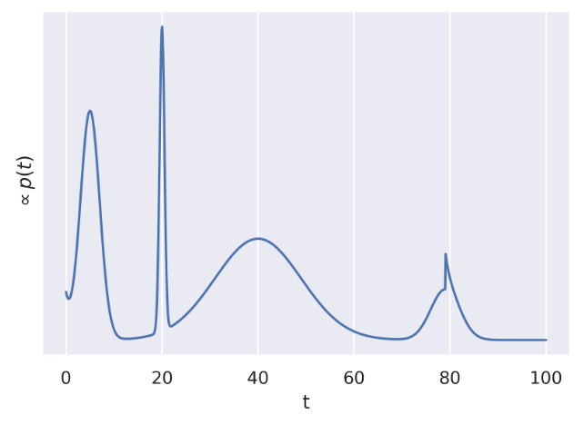Suppose we have four possible proposals to choose from:

• A: uniform distribution of width 1 centered at the current t: Uniform[t-½, t+½]
• B: shifted exponential distribution starting at the current t with lambda=1
• C: normal distribution with mean at the current t and standard deviation 500
• D: normal distribution with mean at the current t and standard deviation 40

In this example:

• B is the worst because it’s impossible to sample values from smaller $t$ than the current value.
• A is poor because it will take a long time to converge.
• C is poor because many proposals will be rejected.
• D is the best because it allows us to generate samples across the entirety of the domain without having too many rejections.