Hypothesis Testing

Hypothesis Testing #

Hypothesis testing is a form of binary decision making (do we accept or reject the null hypothesis?).

Formulate null hypothesis, alternate hypothesis, and test statistic
Compute value of test statistic based on data
Simulate test statistic under null hypothesis many times
Compare results to determine likelihood of result

As an example of how this relates to binary decision making:

Null hypothesis true: reality = 0
Alternative hypothesis true: reality = 1
Fail to reject null: decision = 0
Reject null: decision = 1 So if the null hypothesis is actually true but we end up rejecting it, then a false positive result has occurred.

P Value #

The P-value is the chance if the null hypothesis is true, that the test statistic is equal to or more extreme than the value observed in the data.

If the null hypothesis is actually true, then the probability of obtaining any particular p-value follows a uniform distribution.

Making decision from P-values #

Null Hypothesis Testing #

Null hypothesis statistical testing (NHST): choose a p-value threshold, and see whether p-value is above or below it.

If above: fail to reject; if below: reject null hypothesis
Issue: if we choose $p = 0.05$, we should expect that 1 in 20 tests will have a false positive result ( https://xkcd.com/882/).
This is linked to the replication crisis (scientists pick and choose one test out of many, which increases the likelihood that it is a false positive).
Choosing the threshold = balancing false positives and false negatives. This tradeoff is context dependent.
- Larger threshold = fewer false negatives, more false positives (we don’t actually know in most cases though) 400

Multiple Hypothesis Testing #

When conducting multiple NHST’s, we need a way to measure an error rate that’s related to all of the tests (since we’re likely to see false positives).

There are two rates that we can use:

Family Wise Error Rate (FWER) : the probability that there is at least one FP over all tests
- Factors in randomness from dataset selection over entire population
False Discovery Rate (FDR) : the expectation of the FDP

So what do FWER and FDR actually mean? How are they different? Intuitively, FWER is a lot more conservative than FDR, because it encodes the probability that even a single test out of potentially millions creates a false positive. As a result, if we want a small FWER threshold, we’d probably have to make a lot of false negatives.

FWER is good for use cases where making a false positive error is really bad (e.g. missile detection, where FP = launch missile by accident, start nuclear war).

On the other hand, FDR describes the expected proportion of discoveries that are wrong. FDR is good for use cases where the act of discovering something is more impactful than any false positives or negatives that come out of false discoveries. As an example, UX testing would use FDR since we’d rather detect all possible changes that could improve a user’s experience, even if some don’t actually do anything.

Bonferroni Correction #

Bonferroni correction is a way to control the FWER. The main principle is that we use a fixed $p$ value, and set a threshold $\alpha$. We’d like FWER $\le \alpha$.

Define an indicator variable $E_i$, which is $1$ if test $i$ is a false positive, 0 otherwise. Then, FWER = $P(\bigcup_{i=1}^m E_i)$ (probability that $E_1 = 1$ or $E_2 = 1$ … or $E_m = 1$ )

We can use Boole’s inequality to say that $P(\bigcup_{i=1}^m E_i) \le \sum_{i=1}^m P(E_i)$ (i.e. union is at most the sum of individual probabilities, if every event is independent).

If the $p$-value threshold is $a$, then $P(E_i) = a$, and the sum of $m$ tests is therefore $ma$. So, $\alpha = ma$ which suggests that if we want FWER $\le \alpha$, then we can choose the p-value threshold $\frac{\alpha}{m}$.

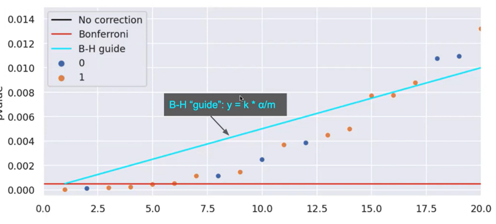
Benjamini-Hochberg Formula #

B-H is used to control the False Discovery Rate. (recall that FDR is the expected value of the proportion of incorrect decisions out of those the algorithm detected to be true.)

General steps:

Sort p-values indexed by k
1. Smallest p-value has $k=1$ and largest has $k=m$
Draw the line $y = k \cdot \alpha/m$
Find the largest p-value under the line and use this as the threshold

In the below example, we would set the B-H threshold to around .008, since that’s where the biggest p-value exists still under the line.

Proof of Benjamini-Hochberg: why does B-H control FDR?

Recall that $FDR = E[FDP] = E[P(R=0|D=1)$. Using Bayes’ rule we can expand $P(R=0|D=1) = \frac{P(D=1|R=0)P(R=0)}{P(D=1)}$.

Define the following quantities:

$m$ = number of tests
$m_0$ = number of true nulls
$k^*$ = index of last p-value below the line
$\alpha^$ = value of line (not p-value) at $k^$

We want to show that $FDR \le \alpha$.

Let’s start by making some substitutions:

$P(R=0) = \frac{m_0}{m}$ (probability that reality is null)
$P(D=1) = \frac{k^*}{m}$ (all tests greater than p-value threshold are classified as 1)
$P(D=1|R=0)$ = p-value $\le \alpha^*$ by B-H

Putting this all together, we get this: $$FDP \le \frac{\alpha^* \cdot \frac{m_0}{m}}{\frac{k^}{m}}$$ which simplifies to $$FDP \le \frac{\alpha^}{k^} \cdot m_0$$ where $\frac{\alpha^}{k^}$ is the slope of the line. Since $k^$ is an index and is thus always at most the last test index $m$, $FDP \le \frac{\alpha}{m} \cdot m_0$. In turn, we know that $m_0 \le m$ so $FDP \le \alpha$, which demonstrates a relationship between FDP and the $\alpha$ treshold determined using B-H.

Online Decision-Making #

Sometimes, we must make decisions as the data comes in. We don’t see all the data upfront, and current decisions may influence future ones.

Intuitively, if we see a lot of small p-values and then an ambigous p-value, we should be more likely to make a D=1 decision. On the other hand, if we see a lot of large p-values and then the same p-value, we should make a D=0 decision instead.

One example of online decision making is A/B tests, where we might want to change the website after 100 users view it, rather than waiting for all 1000 for the test to complete.

If we know the total number of tests, Bonferroni correction can be used to get FWER. However, we can’t use B-H because we need to sort all of the tests’ p-values before making a decision about the threshold.

LORD Procedure #

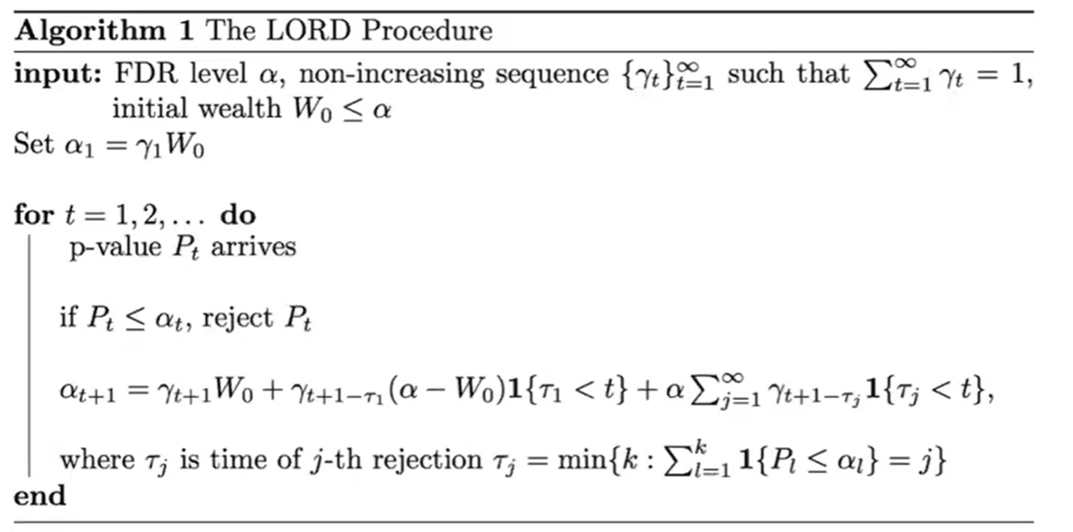
Breaking down this algorithm:

$\gamma_t$ gets smaller (decays) over time.
$\alpha$ is some FDR value we’d like this decision-making process to achieve. At each timestep, we’ll adjust $\alpha$ based on the new values.
At each iteration, we’ll sum over all rejections so far and weight this value by both $\alpha$ and $\gamma_t$. The further away a discovery is from the current time, the more decayed its value is (so it’s worth less in the calculation).
As more discoveries are made, the threshold $\alpha_t$ should increase.
The p-value threshold is known as the “wealth”, and encodes how optimistic we are. The higher the wealth, the easier it is to make a discovery.

Basic summary of LORD: at each timestep, update $\alpha$ by multiplying the decay function with the original weight, and adding this to $\alpha$ multiplied by all timesteps with a rejection, weighted by the difference between the current timestep and the time of rejection. Then, compare the current $\alpha$ value to the p-value obtained to make a decision about whether or not to reject.

Neyman-Pearson Framework #

If we have a defined distribution for both the null and alternative hypotheses, we can define the likelihood ratio to be the probability of getting the test statistic given that the alternative is true, divided by the probability of getting the test statistic given that the null is true.